Month: June 2019

DeepTrading with Tensorflow IV

2019-06-232019-06-24
by parrondo

After you have trained a neural network (NN), you would want to save it for future calculation and eventually deploying to production. So, what is a Tensorflow model? Tensorflow model contains the network design or graph and values of the network parameters that we have trained.

Important Note: I know that the reader is impatient to use real data from the financial markets. Please be patient, I promise that we will use them properly when you are ready, but now we must strengthen our knowledge to have a strong foundation.

Also, remember to have a look at the first posts of the series to have the full picture:

https://todotrader.com/deeptrading-with-tensorflow/

https://todotrader.com/deeptrading-with-tensorflow-ii/

https://todotrader.com/deeptrading-with-tensorflow-iii/

Implementing a one hidden layer Neural Network with save and restore

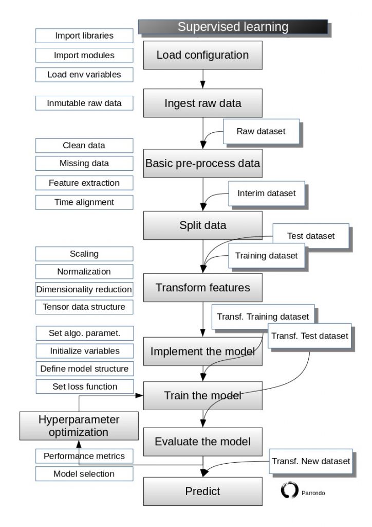
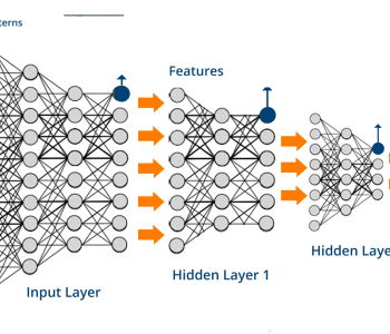
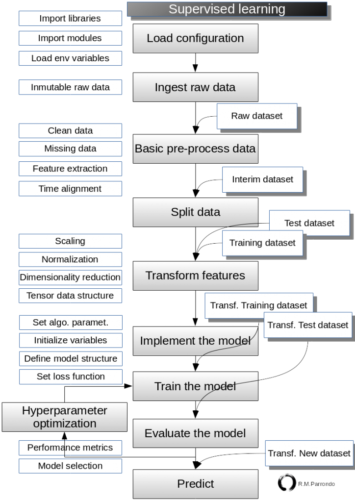
Here is the one-hidden layer network model again to refresh our knowledge. As usual, we will follow our supervised learning flowchart.

The progress of the model can be saved during and after training. This means that a model can be resumed where it left off and avoid long training times. Saving also means that you can share your model and others can recreate your work.

We will illustrate how to create a one hidden layer NN, save it and make predictions with a trained model after reloading it.

Again, we will use the iris data for this exercise. Remember the important note above!

We will build a one-hidden layer neural network to predict the fourth attribute, Petal Width from the other three (Sepal length, Sepal width, Petal length).

There are several differences with respect to the example before in order to illustrate more Tensorflow possibilities.

Caution: TensorFlow model files are code. Be careful with untrusted code. See Using TensorFlow Securely for details.

Load configuration

In [1]:

import matplotlib.pyplot as plt
import numpy as np
import tensorflow as tf
from sklearn.datasets import load_iris
from tensorflow.python.framework import ops
import pandas as pd

/home/parrondo/anaconda3/envs/deeptrading/lib/python3.5/importlib/_bootstrap.py:222: RuntimeWarning: numpy.dtype size changed, may indicate binary incompatibility. Expected 96, got 88
  return f(*args, **kwds)
/home/parrondo/anaconda3/envs/deeptrading/lib/python3.5/importlib/_bootstrap.py:222: RuntimeWarning: numpy.dtype size changed, may indicate binary incompatibility. Expected 96, got 88
  return f(*args, **kwds)
/home/parrondo/anaconda3/envs/deeptrading/lib/python3.5/importlib/_bootstrap.py:222: RuntimeWarning: numpy.dtype size changed, may indicate binary incompatibility. Expected 96, got 88
  return f(*args, **kwds)
/home/parrondo/anaconda3/envs/deeptrading/lib/python3.5/importlib/_bootstrap.py:222: RuntimeWarning: numpy.dtype size changed, may indicate binary incompatibility. Expected 96, got 88
  return f(*args, **kwds)

Ingest raw data

In [2]:

# Before getting into pandas dataframes we will load an example dataset from sklearn library 
# type(data) #iris is a bunch instance which is inherited from dictionary
data = load_iris() #load iris dataset

# We get a pandas dataframe to better visualize the datasets
df = pd.DataFrame(data.data, columns=data.feature_names)

X_raw = np.array([x[0:3] for x in data.data])
y_raw = np.array([x[3] for x in data.data])

# Dimensions of dataset
print("Dimensions of dataset")
n = X_raw.shape[0]
p = X_raw.shape[1]
print("n=",n,"p=",p)

Dimensions of dataset
n= 150 p= 3

In [3]:

data.keys() #keys of the dictionary

Out[3]:

dict_keys(['target_names', 'target', 'data', 'DESCR', 'feature_names'])

In [4]:

X_raw.shape # Array 150x3. Each element is a 3-dimensional data point: sepal length, sepal width, petal length

Out[4]:

(150, 3)

In [5]:

y_raw.shape # Vector 150. Each element is a 1-dimensional (scalar) data point: petal width

Out[5]:

(150,)

In [6]:

df

Out[6]:

	sepal length (cm)	sepal width (cm)	petal length (cm)	petal width (cm)
0	5.1	3.5	1.4	0.2
1	4.9	3.0	1.4	0.2
2	4.7	3.2	1.3	0.2
3	4.6	3.1	1.5	0.2
4	5.0	3.6	1.4	0.2
5	5.4	3.9	1.7	0.4
6	4.6	3.4	1.4	0.3
7	5.0	3.4	1.5	0.2
8	4.4	2.9	1.4	0.2
9	4.9	3.1	1.5	0.1
10	5.4	3.7	1.5	0.2
11	4.8	3.4	1.6	0.2
12	4.8	3.0	1.4	0.1
13	4.3	3.0	1.1	0.1
14	5.8	4.0	1.2	0.2
15	5.7	4.4	1.5	0.4
16	5.4	3.9	1.3	0.4
17	5.1	3.5	1.4	0.3
18	5.7	3.8	1.7	0.3
19	5.1	3.8	1.5	0.3
20	5.4	3.4	1.7	0.2
21	5.1	3.7	1.5	0.4
22	4.6	3.6	1.0	0.2
23	5.1	3.3	1.7	0.5
24	4.8	3.4	1.9	0.2
25	5.0	3.0	1.6	0.2
26	5.0	3.4	1.6	0.4
27	5.2	3.5	1.5	0.2
28	5.2	3.4	1.4	0.2
29	4.7	3.2	1.6	0.2
…	…	…	…	…
120	6.9	3.2	5.7	2.3
121	5.6	2.8	4.9	2.0
122	7.7	2.8	6.7	2.0
123	6.3	2.7	4.9	1.8
124	6.7	3.3	5.7	2.1
125	7.2	3.2	6.0	1.8
126	6.2	2.8	4.8	1.8
127	6.1	3.0	4.9	1.8
128	6.4	2.8	5.6	2.1
129	7.2	3.0	5.8	1.6
130	7.4	2.8	6.1	1.9
131	7.9	3.8	6.4	2.0
132	6.4	2.8	5.6	2.2
133	6.3	2.8	5.1	1.5
134	6.1	2.6	5.6	1.4
135	7.7	3.0	6.1	2.3
136	6.3	3.4	5.6	2.4
137	6.4	3.1	5.5	1.8
138	6.0	3.0	4.8	1.8
139	6.9	3.1	5.4	2.1
140	6.7	3.1	5.6	2.4
141	6.9	3.1	5.1	2.3
142	5.8	2.7	5.1	1.9
143	6.8	3.2	5.9	2.3
144	6.7	3.3	5.7	2.5
145	6.7	3.0	5.2	2.3
146	6.3	2.5	5.0	1.9
147	6.5	3.0	5.2	2.0
148	6.2	3.4	5.4	2.3
149	5.9	3.0	5.1	1.8

150 rows × 4 columns

Basic pre-process data

In [7]:

#
# Leave in blanck intentionally
#

Split data

In [8]:

# split into train and test sets

# Total samples
nsamples = n

# Splitting into train (70%) and test (30%) sets
split = 70 # training split% ; test (100-split)%
jindex = nsamples*split//100 # Index for slicing the samples

# Samples in train
nsamples_train = jindex

# Samples in test
nsamples_test = nsamples - nsamples_train
print("Total number of samples: ",nsamples,"\nSamples in train set: ", nsamples_train,
      "\nSamples in test set: ",nsamples_test)

# Here are train and test samples
X_train = X_raw[:jindex, :]
y_train = y_raw[:jindex]

X_test = X_raw[jindex:, :]
y_test = y_raw[jindex:]

print("X_train.shape = ", X_train.shape, "y_train.shape =", y_train.shape, "\nX_test.shape =  ",
      X_test.shape, "y_test.shape = ", y_test.shape)

Total number of samples:  150 
Samples in train set:  105 
Samples in test set:  45
X_train.shape =  (105, 3) y_train.shape = (105,) 
X_test.shape =   (45, 3) y_test.shape =  (45,)

Transform features

Note

Be careful do not to write X_test_std = sc.fit_transform(X_test) instead of X_test_std = sc.transform(X_test). In this case, it wouldn’t make a great difference since the mean and standard deviation of the test set should be (quite) similar to the training set. However, this is not always the case in Forex market data, as has been well established in the literature. The correct way is to re-use parameters from the training set if we are doing any kind of transformation. So, the test set should basically stand for “new, unseen” data. In [9]:

# Scale data
from sklearn.preprocessing import StandardScaler

sc = StandardScaler()
X_train_std = sc.fit_transform(X_train)
X_test_std = sc.transform(X_test)

y_train_std = sc.fit_transform(y_train.reshape(-1, 1))
y_test_std = sc.transform(y_test.reshape(-1, 1))

Implement the model

In [10]:

# Clears the default graph stack and resets the global default graph
ops.reset_default_graph()

In [11]:

# make results reproducible
seed = 2
tf.set_random_seed(seed)
np.random.seed(seed)  


# Parameters
learning_rate = 0.005
batch_size = 50
n_features = X_train.shape[1]#  Number of features in training data
epochs = 1000
display_step = 50
model_path = "/tmp/model.ckpt"
n_classes = 1

# Network Parameters
# See figure of the model
d0 = D = n_features # Layer 0 (Input layer number of features)
d1 = 10 # Layer 1 (1st hidden layer number of features. Selected 10 for this example)
d2 = C = 1 # Layer 2 (Output layer)

# tf Graph input
print("Placeholders")
X = tf.placeholder(dtype=tf.float32, shape=[None, n_features], name="X")
y = tf.placeholder(dtype=tf.float32, shape=[None,n_classes], name="y")


# Initializers
print("Initializers")
sigma = 1
weight_initializer = tf.variance_scaling_initializer(mode="fan_avg", distribution="uniform", scale=sigma)
bias_initializer = tf.zeros_initializer()

# Create model
def onelayer_perceptron(X, variables):
    # Hidden layer with ReLU activation
    layer_1 = tf.nn.relu(tf.add(tf.matmul(X, variables['W1']), variables['bias1']))
    # Output layer with ReLU activation
    out_layer = tf.nn.relu(tf.add(tf.matmul(layer_1, variables['W2']), variables['bias2']))
    return out_layer

# Store layers weight & bias
variables = {
    'W1': tf.Variable(weight_initializer([n_features, d1]), name="W1"), # inputs -> hidden neurons
    'bias1': tf.Variable(bias_initializer([d1]), name="bias1"), # one biases for each hidden neurons
    'W2': tf.Variable(weight_initializer([d1, d2]), name="W2"), # hidden inputs -> 1 output
    'bias2': tf.Variable(bias_initializer([d2]), name="bias2") # 1 bias for the output
}

# Construct model
y_hat = onelayer_perceptron(X, variables)

# Define loss and optimizer
loss = tf.reduce_mean(tf.square(y - y_hat)) # MSE
optimizer = tf.train.GradientDescentOptimizer(learning_rate).minimize(loss) # Train step

# Initialize the variables (i.e. assign their default value)
init = tf.global_variables_initializer()

# 'Saver' op to save and restore all the variables
saver = tf.train.Saver()

Placeholders
Initializers

Train the model and Evaluate the model

In [12]:

# Running first session
print("Starting 1st session...")
with tf.Session() as sess:

    # Writer to record image, scalar, histogram and graph for display in tensorboard
    writer = tf.summary.FileWriter("/tmp/tensorflow_logs", sess.graph)  # create writer
    writer.add_graph(sess.graph)

    # Run the initializer
    sess.run(init)

    # Training cycle
    train_loss = []
    test_loss = []
    
    for epoch in range(epochs):
        rand_index = np.random.choice(len(X_train), size=batch_size)
        X_rand = X_train[rand_index]
        y_rand = np.transpose([y_train[rand_index]])
        sess.run(optimizer, feed_dict={X: X_rand, y: y_rand})

        train_temp_loss = sess.run(loss, feed_dict={X: X_rand, y: y_rand})
        train_loss.append(np.sqrt(train_temp_loss))
    
        test_temp_loss = sess.run(loss, feed_dict={X: X_test, y: np.transpose([y_test])})
        test_loss.append(np.sqrt(test_temp_loss))
        if (epoch+1) % display_step == 0:
            print("Epoch:", '%04d' % (epoch+1), "Lost=", \
                "{:.9f}".format(train_temp_loss))

    # Close writer
    writer.flush()
    writer.close()
        
    # Save model weights to disk
    save_path = saver.save(sess, model_path)
    print("Model saved in file: %s" % save_path)
    print("First Optimization Finished!")

Starting 1st session...
Epoch: 0050 Lost= 0.599382699
Epoch: 0100 Lost= 0.200652853
Epoch: 0150 Lost= 0.082070500
Epoch: 0200 Lost= 0.046969157
Epoch: 0250 Lost= 0.033277217
Epoch: 0300 Lost= 0.029509921
Epoch: 0350 Lost= 0.046582703
Epoch: 0400 Lost= 0.051407199
Epoch: 0450 Lost= 0.080046408
Epoch: 0500 Lost= 0.032044422
Epoch: 0550 Lost= 0.028484538
Epoch: 0600 Lost= 0.030885572
Epoch: 0650 Lost= 0.053837571
Epoch: 0700 Lost= 0.030355027
Epoch: 0750 Lost= 0.030203044
Epoch: 0800 Lost= 0.021480566
Epoch: 0850 Lost= 0.011752291
Epoch: 0900 Lost= 0.040840883
Epoch: 0950 Lost= 0.035907771
Epoch: 1000 Lost= 0.042663313
Model saved in file: /tmp/model.ckpt
First Optimization Finished!

In [13]:

%matplotlib inline
# Plot loss (MSE) over time
plt.plot(train_loss, 'k-', label='Train Loss')
plt.plot(test_loss, 'r--', label='Test Loss')
plt.title('Loss (MSE) per Generation')
plt.legend(loc='upper right')
plt.xlabel('Generation')
plt.ylabel('Loss')
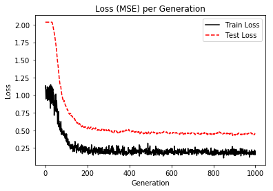
plt.show()

Tensorboard Graph

What follows is the graph we have executed and all the data about it. Note the “save” label.

Saving a Tensorflow model

So, now we have our model saved.

Tensorflow model has four main files:

Meta graph: This is a protocol buffer which saves the complete Tensorflow graph; i.e. all variables, operations, collections, etc. This file has a .meta extension.
Two Checkpoint files: they are binary files which contain all the values of the weights, biases, gradients and all the other variables saved. Tensorflow has changed from version 0.11. Instead of a single .ckpt file, we have now two files: .index and .data file that contains our training variables.
Along with thes, Tensorflow also has a file named checkpoint which simply keeps a record of latest checkpoint files saved.

Retrain the model

We can retrain the model as many times as we want to.

In [14]:

# Running a new session
print("Starting 2nd session...")
with tf.Session() as sess:
    # Initialize variables
    sess.run(init)

    # Restore model weights from previously saved model
    saver.restore(sess, model_path)
    print("Model restored from file: %s" % model_path)

    # Resume training
    for epoch in range(epochs*2):
        rand_index = np.random.choice(len(X_train), size=batch_size)
        X_rand = X_train[rand_index]
        y_rand = np.transpose([y_train[rand_index]])
        sess.run(optimizer, feed_dict={X: X_rand, y: y_rand})

        train_temp_loss = sess.run(loss, feed_dict={X: X_rand, y: y_rand})
        train_loss.append(np.sqrt(train_temp_loss))
    
        test_temp_loss = sess.run(loss, feed_dict={X: X_test, y: np.transpose([y_test])})
        test_loss.append(np.sqrt(test_temp_loss))
        if (epoch+1) % display_step == 0:
            print("Epoch:", '%04d' % (epoch+1), "Lost=", \
                "{:.9f}".format(train_temp_loss))

    # Close writer
    writer.flush()
    writer.close()
    
    # Save model weights to disk
    save_path = saver.save(sess, model_path)
    print("Model saved in file: %s" % save_path)
    print("Second Optimization Finished!")

Starting 2nd session...
INFO:tensorflow:Restoring parameters from /tmp/model.ckpt
Model restored from file: /tmp/model.ckpt
Epoch: 0050 Lost= 0.045188859
Epoch: 0100 Lost= 0.035137746
Epoch: 0150 Lost= 0.040114976
Epoch: 0200 Lost= 0.040839382
Epoch: 0250 Lost= 0.029388864
Epoch: 0300 Lost= 0.050860386
Epoch: 0350 Lost= 0.023227667
Epoch: 0400 Lost= 0.034531657
Epoch: 0450 Lost= 0.036823772
Epoch: 0500 Lost= 0.020957258
Epoch: 0550 Lost= 0.023199901
Epoch: 0600 Lost= 0.029416963
Epoch: 0650 Lost= 0.028286777
Epoch: 0700 Lost= 0.029708408
Epoch: 0750 Lost= 0.038849130
Epoch: 0800 Lost= 0.021901334
Epoch: 0850 Lost= 0.019867409
Epoch: 0900 Lost= 0.038035385
Epoch: 0950 Lost= 0.046836123
Epoch: 1000 Lost= 0.024480129
Epoch: 1050 Lost= 0.025052661
Epoch: 1100 Lost= 0.028433315
Epoch: 1150 Lost= 0.022785973
Epoch: 1200 Lost= 0.018632039
Epoch: 1250 Lost= 0.024766553
Epoch: 1300 Lost= 0.027888060
Epoch: 1350 Lost= 0.030560365
Epoch: 1400 Lost= 0.041359652
Epoch: 1450 Lost= 0.015819877
Epoch: 1500 Lost= 0.029382044
Epoch: 1550 Lost= 0.034098670
Epoch: 1600 Lost= 0.025412932
Epoch: 1650 Lost= 0.036478702
Epoch: 1700 Lost= 0.030148495
Epoch: 1750 Lost= 0.016189585
Epoch: 1800 Lost= 0.023110745
Epoch: 1850 Lost= 0.029191718
Epoch: 1900 Lost= 0.018225947
Epoch: 1950 Lost= 0.023598077
Epoch: 2000 Lost= 0.015231807
Model saved in file: /tmp/model.ckpt
Second Optimization Finished!

Predict

We got it!

Finally, we can use the model to make some predictions.

In [15]:

# Running a new session for predictions
print("Starting prediction session...")
with tf.Session() as sess:
    # Initialize variables
    sess.run(init)

    # Restore model weights from previously saved model
    saver.restore(sess, model_path)
    print("Model restored from file: %s" % model_path)

    # We try to predict the petal width (cm) of three samples
    #Caution!!! This data are not the right data (see below why)
    feed_dict = {X: [[5.1, 3.5, 1.4],
                     [4.8, 3.0, 1.4],
                     [6.3, 3.4, 5.6]]
                }
    prediction = sess.run(y_hat, feed_dict)
    print(prediction) # True value 0.2, 0.1, 2.4

Starting prediction session...
INFO:tensorflow:Restoring parameters from /tmp/model.ckpt
Model restored from file: /tmp/model.ckpt
[[0.19734718]
 [0.28260154]
 [1.7156498 ]]

Caution Note: continue reading

OK, not very good results. But it is worst that we could think! Data are not right because we have trained our model with transformed data (standardization) and now we must use again transformed data to make predictions. Also, we will get back-transformed data again. So, we must inverse the transformation to get the original kind of data.

First: transform our original data. The data we want to make the prediction about.

In [16]:

X_pred = [[5.1, 3.5, 1.4],
          [4.8, 3.0, 1.4],
          [6.3, 3.4, 5.6]]

In [17]:

X_pred_std = sc.transform(X_pred)
X_pred_std

Out[17]:

array([[6.86549436, 4.28228483, 0.89182234],
       [6.38114257, 3.47503186, 0.89182234],
       [8.8029015 , 4.12083424, 7.67274733]])

Second: we are ready to make the predictions

In [18]:

# Running a new session for predictions
print("Starting prediction session...")
with tf.Session() as sess:
    # Initialize variables
    sess.run(init)

    # Restore model weights from previously saved model
    saver.restore(sess, model_path)
    print("Model restored from file: %s" % model_path)

    # We try to predict the petal width (cm) of three samples
    feed_dict_std = {X: [[6.86549436, 4.28228483, 0.89182234],
       [6.38114257, 3.47503186, 0.89182234],
       [8.8029015 , 4.12083424, 7.67274733]]}
    prediction = sess.run(y_hat, feed_dict_std)
    print(prediction) # True value 0.2, 0.1, 2.4

Starting prediction session...
INFO:tensorflow:Restoring parameters from /tmp/model.ckpt
Model restored from file: /tmp/model.ckpt
[[0.15292837]
 [0.20799588]
 [2.3737454 ]]

Third: we reverse the transformation

In [19]:

y_hat_rev = sc.inverse_transform(prediction)
y_hat_rev

Out[19]:

array([[0.9423405],
       [0.9764485],
       [2.3178802]], dtype=float32)

Not bad. True values are 0.2, 0.1, 2.4. We’ll try to improve them with a deeper network. That is the goal of the next notebook.

In the mean time, try to have a full comprehension of this result.

Remember you can get the full Jupyter notebook on my Github repo:

https://github.com/parrondo/deeptrading

Black Belt

DeepTrading with TensorFlow III

2019-06-192019-06-22
by parrondo

We are now closer to applying our knowledge of neural networks (NN) to our trading systems. But, we still have to tune our rudiments a bit on TensorFlow.
If you are not yet familiar with our supervised machine learning flowchart, take a look at the first two posts in this series.

DeepTrading with Tensorflow

DeepTrading with TensorFlow II

As usual, the calculations contained in this post are part of a Jupyter notebook that is in our Github repository:

https://github.com/parrondo/deeptrading

Implementing a one hidden layer Neural Network

We will illustrate how to create a one hidden layer NN.

The readers will use the iris data for this exercise.

Finally, we will build a one-hidden-layer neural network to predict the fourth attribute, Petal Width from the other three (Sepal length, Sepal width, Petal length).

Load configuration

In [1]:

import matplotlib.pyplot as plt
import numpy as np
import tensorflow as tf
from sklearn.datasets import load_iris
from tensorflow.python.framework import ops
import pandas as pd

Ingest raw data

In [2]:

# Before getting into pandas dataframes we will load an example dataset from sklearn library 
# type(data) #iris is a bunch instance which is inherited from dictionary
data = load_iris() #load iris dataset



data = load_iris()

# We get a pandas dataframe to better visualize the datasets
df = pd.DataFrame(data.data, columns=data.feature_names)

X_raw = np.array([x[0:3] for x in data.data])
y_raw = np.array([x[3] for x in data.data])

# Dimensions of dataset
print("Dimensions of dataset")
n = X_raw.shape[0]
p = X_raw.shape[1]
print("n=",n,"p=",p)

Dimensions of dataset
n= 150 p= 3

In [3]:

data.keys() #keys of the dictionary

Out[3]:

dict_keys(['DESCR', 'data', 'target', 'feature_names', 'target_names'])

In [4]:

X_raw.shape # Array 150x3. Each element is a 3-dimensional data point: sepal length, sepal width, petal length

Out[4]:

(150, 3)

In [5]:

y_raw.shape # Vector 150. Each element is a 1-dimensional (scalar) data point: petal width

Out[5]:

(150,)

In [6]:

df

Out[6]:

	sepal length (cm)	sepal width (cm)	petal length (cm)	petal width (cm)
0	5.1	3.5	1.4	0.2
1	4.9	3.0	1.4	0.2
2	4.7	3.2	1.3	0.2
3	4.6	3.1	1.5	0.2
4	5.0	3.6	1.4	0.2
5	5.4	3.9	1.7	0.4
6	4.6	3.4	1.4	0.3
7	5.0	3.4	1.5	0.2
8	4.4	2.9	1.4	0.2
9	4.9	3.1	1.5	0.1
10	5.4	3.7	1.5	0.2
11	4.8	3.4	1.6	0.2
12	4.8	3.0	1.4	0.1
13	4.3	3.0	1.1	0.1
14	5.8	4.0	1.2	0.2
15	5.7	4.4	1.5	0.4
16	5.4	3.9	1.3	0.4
17	5.1	3.5	1.4	0.3
18	5.7	3.8	1.7	0.3
19	5.1	3.8	1.5	0.3
20	5.4	3.4	1.7	0.2
21	5.1	3.7	1.5	0.4
22	4.6	3.6	1.0	0.2
23	5.1	3.3	1.7	0.5
24	4.8	3.4	1.9	0.2
25	5.0	3.0	1.6	0.2
26	5.0	3.4	1.6	0.4
27	5.2	3.5	1.5	0.2
28	5.2	3.4	1.4	0.2
29	4.7	3.2	1.6	0.2
…	…	…	…	…
120	6.9	3.2	5.7	2.3
121	5.6	2.8	4.9	2.0
122	7.7	2.8	6.7	2.0
123	6.3	2.7	4.9	1.8
124	6.7	3.3	5.7	2.1
125	7.2	3.2	6.0	1.8
126	6.2	2.8	4.8	1.8
127	6.1	3.0	4.9	1.8
128	6.4	2.8	5.6	2.1
129	7.2	3.0	5.8	1.6
130	7.4	2.8	6.1	1.9
131	7.9	3.8	6.4	2.0
132	6.4	2.8	5.6	2.2
133	6.3	2.8	5.1	1.5
134	6.1	2.6	5.6	1.4
135	7.7	3.0	6.1	2.3
136	6.3	3.4	5.6	2.4
137	6.4	3.1	5.5	1.8
138	6.0	3.0	4.8	1.8
139	6.9	3.1	5.4	2.1
140	6.7	3.1	5.6	2.4
141	6.9	3.1	5.1	2.3
142	5.8	2.7	5.1	1.9
143	6.8	3.2	5.9	2.3
144	6.7	3.3	5.7	2.5
145	6.7	3.0	5.2	2.3
146	6.3	2.5	5.0	1.9
147	6.5	3.0	5.2	2.0
148	6.2	3.4	5.4	2.3
149	5.9	3.0	5.1	1.8

150 rows × 4 columns

Basic pre-process data

Here we will do nothing, but I like to leave it blank so that the reader does not lose the thread of our flowchart. 🙂

In [7]:

#
# Leave in blanck intentionally
#

Split data

In [8]:

# split into train and test sets

# Total samples
nsamples = n

# Splitting into train (70%) and test (30%) sets
split = 70 # training split% ; test (100-split)%
jindex = nsamples*split//100 # Index for slicing the samples

# Samples in train
nsamples_train = jindex

# Samples in test
nsamples_test = nsamples - nsamples_train
print("Total number of samples: ",nsamples,"\nSamples in train set: ", nsamples_train,
      "\nSamples in test set: ",nsamples_test)

# Here are train and test samples
X_train = X_raw[:jindex, :]
y_train = y_raw[:jindex]

X_test = X_raw[jindex:, :]
y_test = y_raw[jindex:]

print("X_train.shape = ", X_train.shape, "y_train.shape =", y_train.shape, "\nX_test.shape =  ",
      X_test.shape, "y_test.shape = ", y_test.shape)

Total number of samples:  150 
Samples in train set:  105 
Samples in test set:  45
X_train.shape =  (105, 3) y_train.shape = (105,) 
X_test.shape =   (45, 3) y_test.shape =  (45,)

Transform features

Important Note

Be careful not to writeX_test_std = sc.fit_transform(X_test) instead ofX_test_std = sc.transform(X_test). In this case, it wouldn’t make a great difference since the mean and standard deviation of the test set should be (quite) similar to the training set. However, this is not always the case in Forex market data, as has been well established in the literature. The correct way is to re-use parameters from the training set if we are doing any kind of transformation. So, the test set should basically stand for “new, unseen” data.

In [9]:

# Scale data
from sklearn.preprocessing import StandardScaler

sc = StandardScaler()
X_train_std = sc.fit_transform(X_train)
X_test_std = sc.transform(X_test)

y_train_std = sc.fit_transform(y_train.reshape(-1, 1))
y_test_std = sc.transform(y_test.reshape(-1, 1))

Implement the model

In [10]:

# Clears the default graph stack and resets the global default graph
ops.reset_default_graph()

In [11]:

# make results reproducible
seed = 2
tf.set_random_seed(seed)
np.random.seed(seed)  

# Initialize hyperparameters
n_features = X_train.shape[1]#  Number of features in training data
print("Number of featuress in training data: ", n_features)

batch_size = 50

# Placeholders
print("Placeholders")
X = tf.placeholder(dtype=tf.float32, shape=[None, n_features], name="X")
y = tf.placeholder(dtype=tf.float32, shape=[None,1], name="y")

# Initializers
print("Initializers")
sigma = 1
weight_initializer = tf.variance_scaling_initializer(mode="fan_avg", distribution="uniform", scale=sigma)
bias_initializer = tf.zeros_initializer()

Number of featuress in training data:  3
Placeholders
Initializers

In [12]:

# Dimensions of the layers (aka layer nodes, neurons)(See figure of the model)
d0 = D = n_features # Layer 0 (Input layer)
d1 = 10 # Layer 1 (Hidden layer 1). Selected 10 for this example
d2 = C = 1 # Layer 2 (Output layer)

print("d0 =", d0, "d1 =", d1, "d2 =", d2)

# Create variables for NN layers
W1 = tf.Variable(weight_initializer([n_features, d1]), name="W1") # inputs -> hidden neurons
bias1 = tf.Variable(bias_initializer([d1]), name="bias1") # one biases for each hidden neurons
W2 = tf.Variable(weight_initializer([d1, d2]), name="W2") # hidden inputs -> 1 output
bias2 = tf.Variable(bias_initializer([d2]), name="bias2") # 1 bias for the output

# Construct model
hidden_output = tf.nn.relu(tf.add(tf.matmul(X, W1), bias1))
final_output = tf.nn.relu(tf.add(tf.matmul(hidden_output, W2), bias2))

# Define loss function (MSE)
loss = tf.reduce_mean(tf.square(y - final_output))

# Define optimizer
my_opt = tf.train.GradientDescentOptimizer(0.005)
train_step = my_opt.minimize(loss)

# Initialize variables
init = tf.global_variables_initializer()

d0 = 3 d1 = 10 d2 = 1

In [13]:

W1

Out[13]:

<tf.Variable 'W1:0' shape=(3, 10) dtype=float32_ref>

Train the model and Evaluate the model

In [14]:

# Create graph session 
sess = tf.Session()

# Writer to record image, scalar, histogram and graph for display in tensorboard
writer = tf.summary.FileWriter("/tmp/tensorflow_logs", sess.graph)

sess.run(init)

# Training loop
train_loss = []
test_loss = []
for i in range(1000):
    rand_index = np.random.choice(len(X_train), size=batch_size)
    X_rand = X_train[rand_index]
    y_rand = np.transpose([y_train[rand_index]])
    sess.run(train_step, feed_dict={X: X_rand, y: y_rand})

    train_temp_loss = sess.run(loss, feed_dict={X: X_rand, y: y_rand})
    train_loss.append(np.sqrt(train_temp_loss))
    
    test_temp_loss = sess.run(loss, feed_dict={X: X_test, y: np.transpose([y_test])})
    test_loss.append(np.sqrt(test_temp_loss))
    if (i+1)%50==0:
        print('Generation: ' + str(i+1) + '. Loss = ' + str(train_temp_loss))

writer.flush()
writer.close()

Generation: 50. Loss = 0.5993827
Generation: 100. Loss = 0.20065285
Generation: 150. Loss = 0.0820705
Generation: 200. Loss = 0.046969157
Generation: 250. Loss = 0.033277217
Generation: 300. Loss = 0.02950992
Generation: 350. Loss = 0.046582703
Generation: 400. Loss = 0.0514072
Generation: 450. Loss = 0.08004641
Generation: 500. Loss = 0.032044422
Generation: 550. Loss = 0.028484538
Generation: 600. Loss = 0.030885572
Generation: 650. Loss = 0.05383757
Generation: 700. Loss = 0.030355027
Generation: 750. Loss = 0.030203044
Generation: 800. Loss = 0.021480566
Generation: 850. Loss = 0.011752291
Generation: 900. Loss = 0.040840883
Generation: 950. Loss = 0.03590777
Generation: 1000. Loss = 0.042663313

In [15]:

%matplotlib inline
# Plot loss (MSE) over time
plt.plot(train_loss, 'k-', label='Train Loss')
plt.plot(test_loss, 'r--', label='Test Loss')
plt.title('Loss (MSE) per Generation')
plt.legend(loc='upper right')
plt.xlabel('Generation')
plt.ylabel('Loss')
plt.show()

Tensorboard Graph

What follows is the graph we have executed and all data about it.

Predict

In [16]:

#
# Leave in blanck intentionally
#

We have reached the end of this post, but don’t worry, I will continue it very soon.
In the meantime, I propose that you put your infrastructure in place to create trading systems. Take a look at the following posts that are aimed at you acquiring good practices. So, your work could be reproducible.

Quant Trading Project Structure

Robust Git Workflow for Research Projects

Remember all these calculations are included in a Jupyter notebook in my Github repository:

https://github.com/parrondo/deeptrading

Black Belt

DeepTrading with TensorFlow II

2019-06-152019-06-22
by parrondo

OK, you know what tensors are or perhaps you don’t, but you are sure you want to use TensorFlow to trade with it. This post introduces you to how to create elemental NN tensors in TensorFlow.

This is the second post of the serie, so you need to be familiarized with the concepts exposed in the first post DeepTrading with Tensorflow.

Tensors

Tensors (of order higher than two) are data structures indexed by three or more indices, say (i,j,k,…) — a generalization of matrices, which are indexed by two indices, (m,n) for (m rows, n columns). These algebraic animals are very interesting from a theoretical point of view, and tensor-based methods have recently become very important in signal processing, data science, and machine learning applications.

Internally, TensorFlow represents tensors as n-dimensional arrays of base data types.

We use tensors all the time in Deep Learning, but you do not need to be an expert in them to use it. You may need to understand a little about them, so here are some good resources:

How to create elemental NN tensors in TensorFlow

The following is an elemental computational graph that we are going to create and execute. It is very similar to many of the calculations that must be made in artificial neural networks. We will use Jupyter notebook to accomplish all calculations.

It is formed by a linear transformation, xW + b, followed by a non-linear activation fucntion, ReLU(). Where:

x is a D-dimensional data point.
W is the DxM matrix of weights.
b is the bias M-dimensional vector

We will always follow the supervised flowchart:

Remember that you can find the complete Jupyter notebook in my Github repository:

https://github.com/parrondo/deeptrading

LOAD CONFIGURATION

First, we start with loading TensorFlow and resetting the computational graph.

In [1]:

import tensorflow as tf #Tensorflow 1.5 import warnings https://github.com/ContinuumIO/anaconda-issues/issues/6678
from tensorflow.python.framework import ops
ops.reset_default_graph()
import random as rnd
import numpy as np

/home/parrondo/anaconda3/envs/deeptrading/lib/python3.5/importlib/_bootstrap.py:222: RuntimeWarning: numpy.dtype size changed, may indicate binary incompatibility. Expected 96, got 88
  return f(*args, **kwds)
/home/parrondo/anaconda3/envs/deeptrading/lib/python3.5/importlib/_bootstrap.py:222: RuntimeWarning: numpy.dtype size changed, may indicate binary incompatibility. Expected 96, got 88
  return f(*args, **kwds)

IMPLEMENT THE MODEL

1. Build a graph

a. Graph contains parameter specifications, model architecture, optimization process, …
b. Somewhere between 5 and 5000 lines

These are the elements involved in our graph:

Variables are 0-ary stateful nodes which output their current value.
Placeholders are 0-ary nodes whose value is fed in at execution time.
Mathematical operations:
- MatMul: Multiply two matrix values.
- Add: Add elementwise (with broadcasting).
- ReLU: Activate with elementwise rectified linear function.

In [2]:

b = tf.Variable(tf.zeros((100,)), name='biases')
W=tf.Variable(tf.random_uniform((1024, 100), -1, 1), name='weights')
x = tf.placeholder(tf.float32, (1, 1024), name="x")
h_i = tf.nn.relu(tf.matmul(x, W) + b, name="h_i")

Now, you can see what the object b is:

In [3]:

And the output:

Out[3]:

<tf.Variable 'biases:0' shape=(100,) dtype=float32_ref>

The object W:

In [4]:

Out[4]:

<tf.Variable 'weights:0' shape=(1024, 100) dtype=float32_ref>

The object x:

In [5]:

Out[5]:

<tf.Tensor 'x:0' shape=(1, 1024) dtype=float32>

2. Start a graph session

Launch the graph in a session.

a session: a binding to a particular execution context sess.run(fetches, feeds)
Fetches: List of graph nodes. Return the outputs of these nodes.
Feeds: Dictionary mapping from graph nodes to concrete values. Specifies the value of each graph node given in the dictionary.

In [6]:

# Initial and Run Session
sess = tf.Session()
sess.run(tf.global_variables_initializer())
rand_array = np.random.rand(1, 1024)
sess.run(h_i, feed_dict={x: rand_array})

Out[6]:

array([[ 0.        ,  2.3799796 ,  0.        ,  0.        ,  0.        ,
         5.7116704 ,  9.892372  ,  0.        ,  0.        , 10.10139   ,
         0.        ,  0.40419406,  6.433485  ,  8.08982   ,  3.366507  ,
         0.        ,  2.9525614 ,  0.6404748 ,  0.        , 13.50066   ,
         0.        ,  0.        ,  0.        ,  0.        , 11.59197   ,
         0.        ,  0.        ,  7.8827147 , 14.467917  ,  0.        ,
         0.        ,  0.        ,  9.669572  ,  0.0907014 , 16.898396  ,
         0.        ,  0.        ,  3.7823548 ,  0.        ,  0.7162654 ,
         0.        , 17.48152   ,  0.        ,  3.1157236 ,  0.        ,
         1.0707028 ,  0.        ,  0.        ,  0.        ,  6.848372  ,
        11.503601  ,  0.        ,  0.        ,  3.4340348 ,  0.        ,
         1.9381552 ,  3.2755644 ,  6.5616198 , 10.4794655 ,  0.        ,
         1.5994972 ,  0.        ,  0.        ,  0.        ,  0.        ,
         0.        ,  8.973095  , 11.838539  ,  0.        ,  0.5300804 ,
         0.        , 16.315956  ,  8.245536  ,  0.        , 11.83759   ,
         0.        , 14.958574  ,  0.        , 13.71896   , 21.845812  ,
         3.563043  , 16.940338  ,  0.        ,  8.182699  ,  9.952968  ,
         8.413696  , 15.420557  ,  0.        , 12.520411  ,  0.        ,
         8.671607  ,  0.        ,  0.        ,  3.582255  ,  0.        ,
        17.792744  ,  0.        ,  2.5677953 , 12.895992  ,  0.        ]],
      dtype=float32)

Visualizing the Variable Creation in TensorBoard

To visualize the creation of variables in Tensorboard, we will reset the computational graph and create a global initializing operation.

Typical TensorFlow graphs can have many thousands of nodes. To simplify, variable names can be grouped and the visualization uses this information to define a hierarchy on the nodes in the graph. By default, only the top of this hierarchy is shown. Here is an example that defines three operations under the hidden name scope using:tf.name_scope

Grouping nodes by name scopes is important to making a legible graph. If we are building a model, name scopes give us control over the resulting visualization. The better our name scopes, the better our visualization.

In [7]:

# Reset graph
ops.reset_default_graph()

b = tf.Variable(tf.zeros((100,)), name='biases')
W=tf.Variable(tf.random_uniform((1024, 100), -1, 1), name='weights')
x = tf.placeholder(tf.float32, (1, 1024), name="x")
h_i = tf.nn.relu(tf.matmul(x, W) + b, name="h_i")


# Initial and Run Session
with tf.Session() as sess:
    writer = tf.summary.FileWriter("/tmp/tensorflow_logs", sess.graph)
    sess.run(tf.global_variables_initializer())
    rand_array = np.random.rand(1, 1024)
    sess.run(h_i, feed_dict={x: rand_array})
    writer.flush()
    writer.close()

Therefore, we now run the following command in our command prompt:

$ <code>tensorboard --logdir=tmp/tensorflow_logs</code>

And it will tell us the URL we can navigate our browser to see Tensorboard. The default should be:

http://0.0.0.0:6006/

Here is the graph.

graph_1 — Our first TensorFlow graph as view in Tensorboard

Creating Tensors

TensorFlow has built-in function to create tensors for use in variables. For example, we can create a zero-filled tensor of predefined shape using the functiontf.zeros() as follows.

In [8]:

one_tensor = tf.zeros([1,50])

3. Fetch and feed data with Session.run

The Compilation, optimization, etc. are involved in this step. We probably will not notice

We can evaluate tensors by calling a run() method on our session.

In [9]:

# Start session
sess = tf.Session()
sess.run(tf.global_variables_initializer())

sess.run(one_tensor)

Out[9]:

array([[0., 0., 0., 0., 0., 0., 0., 0., 0., 0., 0., 0., 0., 0., 0., 0.,
        0., 0., 0., 0., 0., 0., 0., 0., 0., 0., 0., 0., 0., 0., 0., 0.,
        0., 0., 0., 0., 0., 0., 0., 0., 0., 0., 0., 0., 0., 0., 0., 0.,
        0., 0.]], dtype=float32)

TensorFlow algorithms need to know which objects are variables and which are constants. Therefore, we create a variable using the TensorFlow function: tf.Variable() as follows.

In [10]:

one_var = tf.Variable(tf.zeros([1,64]))

Note that we can not run, sess.run(one_var) this would result in an error. Because TensorFlow operates with computational graphs, we have to create a variable initialization operation in order to evaluate variables. So, we can initialize one variable at a time by calling the variable method, one_var.initializer

In [11]:

sess.run(one_var.initializer)
sess.run(one_var)

Out[11]:

array([[0., 0., 0., 0., 0., 0., 0., 0., 0., 0., 0., 0., 0., 0., 0., 0.,
        0., 0., 0., 0., 0., 0., 0., 0., 0., 0., 0., 0., 0., 0., 0., 0.,
        0., 0., 0., 0., 0., 0., 0., 0., 0., 0., 0., 0., 0., 0., 0., 0.,
        0., 0., 0., 0., 0., 0., 0., 0., 0., 0., 0., 0., 0., 0., 0., 0.]],
      dtype=float32)

It is very important to control the dimensions of our entities. So, this is a very sensitive point and due to the high quantity of data involved in NN calculations, that detail is of major importance. Let’s first start by creating variables of specific shape by declaring our row and column size.

In [12]:

row_dim = 3
col_dim = 5

Here are variables initialized to contain all zeros or ones.

In [13]:

zero_var = tf.Variable(tf.zeros([row_dim, col_dim]))
ones_var = tf.Variable(tf.ones([row_dim, col_dim]))

Now, we can call the initializer method on our variables and run them to evaluate their contents.

In [14]:

sess.run(zero_var.initializer)
sess.run(ones_var.initializer)
print(sess.run(zero_var))
print(sess.run(ones_var))

[[0. 0. 0. 0. 0.]
 [0. 0. 0. 0. 0.]
 [0. 0. 0. 0. 0.]]
[[1. 1. 1. 1. 1.]
 [1. 1. 1. 1. 1.]
 [1. 1. 1. 1. 1.]]

In [15]:

# Type the entity class
zero_var

Out[15]:

<tf.Variable 'Variable_1:0' shape=(3, 5) dtype=float32_ref>

In [16]:

# Type the entity class
ones_var

Out[16]:

<tf.Variable 'Variable_2:0' shape=(3, 5) dtype=float32_ref>

Creating Tensors Based on Other Tensor’s Shape

If the shape of a tensor depends on the shape of another tensor, then we can use the TensorFlow built-in functions, ones_like()or,zeros_like()

In [17]:

other_zero_var = tf.Variable(tf.zeros_like(zero_var))
other_ones_var = tf.Variable(tf.ones_like(ones_var))

sess.run(other_zero_var.initializer)
sess.run(other_ones_var.initializer)

print(sess.run(other_zero_var))
print(sess.run(other_ones_var))

[[0. 0. 0. 0. 0.]
 [0. 0. 0. 0. 0.]
 [0. 0. 0. 0. 0.]]
[[1. 1. 1. 1. 1.]
 [1. 1. 1. 1. 1.]
 [1. 1. 1. 1. 1.]]

Filling a Tensor with a Constant

Here is how we fill a tensor with a constant.

In [18]:

filled_var = tf.Variable(tf.fill([row_dim, col_dim], 3.14))
sess.run(filled_var.initializer)
print(sess.run(filled_var))

[[3.14 3.14 3.14 3.14 3.14]
 [3.14 3.14 3.14 3.14 3.14]
 [3.14 3.14 3.14 3.14 3.14]]

We can also create a variable from an array or list of constants.

In [19]:

# Create a variable from a constant
const_var = tf.Variable(tf.constant([3, 1, 4, 1, 5, 9, 2]))

# This can also be used to fill an array:
const_fill_array = tf.Variable(tf.constant([3,1,4,1,5,9,2,6,5,3,5,8,9,7,9], shape=[row_dim, col_dim]))

sess.run(const_var.initializer)
sess.run(const_fill_array.initializer)

print(sess.run(const_var))
print(sess.run(const_fill_array))

[3 1 4 1 5 9 2]
[[3 1 4 1 5]
 [9 2 6 5 3]
 [5 8 9 7 9]]

Creating Tensors Based on Sequences and Ranges

We can also create tensors from sequence generation functions in TensorFlow. The TensorFlow function, linspace() and, range() operate very similar to the python/numpy equivalents.

In [20]:

# Linspace in TensorFlow
linear_var = tf.Variable(tf.linspace(start=0.0, stop=1.0, num=5)) # Generates [0.,0.25,0.5,0.75, 1.] includes the end

# Range in TensorFlow
sequence_var = tf.Variable(tf.range(start=6, limit=17, delta=3)) # Generates [6, 9, 12, 15] doesn't include the end

sess.run(linear_var.initializer)
sess.run(sequence_var.initializer)

print(sess.run(linear_var))
print(sess.run(sequence_var))

[0.   0.25 0.5  0.75 1.  ]
[ 6  9 12 15]

Random Number Tensors

Certainly, we can initialize tensors that come from random numbers like following. In [21]:

rnorm_var = tf.random_normal([row_dim, col_dim], mean=0.0, stddev=1.0)
runif_var = tf.random_uniform([row_dim, col_dim], minval=0, maxval=4)

print(sess.run(rnorm_var))
print(sess.run(runif_var))

[[-1.3629563  -1.3664439  -0.72835475 -2.3570406  -0.31535667]
 [ 0.26235196  0.301876    0.20770198  2.2769299   1.7364241 ]
 [-0.388656    0.3083807   1.0538763   0.4854179  -0.41834855]]
[[0.67954206 2.5638103  1.9654655  2.6455693  2.5157561 ]
 [0.733438   0.48339128 3.7160473  2.1167154  1.9247737 ]
 [3.7721186  2.155336   2.2508612  3.9784613  3.4868307 ]]

Come on TRY IT! Don’t forget to visit my Github repository to get this series posts related notebooks:

https://github.com/parrondo/deeptrading

Black Belt

DeepTrading with TensorFlow

2019-06-122019-06-22
by parrondo

Do you want to maximize your trading knowledge using TensorFlow? Here are several tips that will surely help you.

Introduction

Within TodoTrader’s commitment related to the generation and dissemination of knowledge, I want to offer a series of tutorials on the use of TensorFlow for algorithmic trading.

The objective of these tutorials, which I will publish periodically, is to offer in a simple and didactic way, through practical examples, the basics and basic concepts essential for the task of algorithmic trading. At the end of the series, we will have developed an application that allows creating a neural network in TensorFlow, trainable and able to perform operations in the financial markets.

How TensorFlow Works

The complexity of the financial markets has forced to create trading strategies based on artificial intelligence (AI) models. The last ones require a large amount of computing and deep learning algorithms can easily need tens of millions of parameters and billions of connections. Algorithmic trading is full of data and calculations with the data. To deal with it, tensors (multidimensional data arrays) are ideal mathematical entities. And Tensorflow is the right software to use tensors. The training and use of those models require enormous computational resources, in addition, the TensorFlow library allows one to concentrate on the creativity of its solution and leave the infrastructure aside.

TensorFlow was open-sourced in November 2015. Since the inception date, TensorFlow has become Github’s most prominent machine learning repository. (https://github.com/tensorflow/tensorflow)

TensorFlow’s popularity is due to many things, but mainly because of the computational graph concept and the adaptability of the Tensorflow python API structure. This makes solving real problems with TensorFlow accessible to most programmers, even the beginner ones.

You can get all these tutorials in my Github repository:

https://github.com/parrondo/deeptrading

How TensorFlow Operates

Basics of TensorFlow is that first, we create a model which is called a computational graph with TensorFlow objects then we create a TensorFlow session in which we start running all the computation. This tutorial will talk you through pseudocode of how a Tensorflow algorithm usually works.

Tensorflow is supported on the three principal OS systems (Windows, Linux, and Mac). Throughout these Jupyter notebooks, we will only concern ourselves with the Python library wrapper of Tensorflow. This book will use Python 3.X (https://www.python.org) and Tensorflow 0.10+ (https://www.tensorflow.org). Tensorflow can run on the CPU, but it runs faster if it runs on the GPU, and it is supported on graphics cards with NVidia Compute Capability 3.0+. To run on a GPU, you will also need to download and install the NVidia Cuda Toolkit (https://developer.nvidia.com/cuda-downloads).

As usual, we use Conda environments to develop our code (https://github.com/parrondo/quant-trading-project-structure). Please look into the file inside the main directory of this repository, environment.yml, and run the command:

$ conda env create --file environment.yml

So you guarantee that all the necessary libraries are available.

Important Note: As I mentioned in my previous post, Build TensorFlow from Source in Centos 7, the binary files of TensorFlow for Linux is only available in Conda for CPU up to version 1.5. Therefore I preferred to limit the notebooks to this version to avoid possible problems for readers. However, these examples have been tested until the stable released version 1.12 working perfectly (compiled by me for CPU).

General TensorFlow Algorithm Workflow

Here we introduce the general workflow of TensorFlow Algorithms. This workflow can be follow as a template.

Load configuration

This is usually the first step. Here you import libraries and modules as needed. Also, load environment variables and configuration files.

Ingest data

All of machine learning algorithms depend on data. So, we either generate data or use an outside source of data. Sometimes it is better to rely on generated data because we will want to test the expected outcome. Most times we will access market data sets for the given research. in any case, it is convenient to have a well defined ingestion data model as we provide in this tutorial.

Output: raw dataset files under “data/raw” folder.

Basic pre-process data

The raw dataset usually has faults which difficult the next steps. In these steps, we proceed to clean data, manage missing data, define features and labels, encode the dependent variable and dataset time alignment when necessary.

Split data

This step is useful when you need to separate data into training and test sets. We can also customize the way to divide the data. Sometimes we need to support data randomization; but, a certain type of data or model type needs the design of other split methods.

Output: two dataset training dataset and test dataset, usually they are resident in memory but in case we need to save them, then “data/interim” is our folder.

Transform features

In general, the data is not in the correct dimension, structure or type expected by our TensorFlow trading algorithms. We have to transform the raw or provisional (interim) data before we can use them. Most algorithms also expect standardized (normalized) data and we will do this here as well. Tensorflow has built-in functions that can normalize the data for you.

  data = tf.nn.batch_norm_with_global_normalization(...)

Caution! Some algorithms require normalization of the data before training a model. Other algorithms, on the other hand, perform their own data scale or normalization. So, when choosing an automatic learning algorithm to use in a predictive model, be sure to review the algorithm data requirements before applying the normalization to the training data.

This stage include dimension reduction, when necessary.

Finally, in this step, we must have clear what will be the structure (dimensions) of the tensors that are involved in the input of data and in all calculations.

Output: two datasets transformed training dataset and transformed test dataset. It may be, this step is accomplished several times given several pairs of train-test datasets (i.e. normalized dataset, PCA dataset, standardized dataset,…)

Implement the model

Several sub-process expected here, describing as follow:

Set algorithm parameters

Algorithms usually have a set of parameters that we hold constant throughout the procedure (i.e. the number of iterations, the learning rate, or other fixed parameters). It is a good practice to initialize these together so the user can easily find them.

learning_rate = 0.005
a = b
iterations = 1000
epochs=50

Initialize variables and placeholders

we have to tell Tensorflow what it can and cannot modify. TensorFlow will modify the variables during optimization to minimize a loss function. To accomplish this, we feed in data through placeholders. Placeholder simply allocates a block of memory for future use. By default, placeholder has an unconstrained shape, which allows us to feed tensors of different shapes in a session. We need to initialize variables and define size and type of placeholders so that TensorFlow knows what to expect.

k_var = tf.constant(50)
x_train = tf.placeholder(tf.float32, [None, input_size])
y_train = tf.placeholder(tf.fload32, [None, num_classes])

Define the model structure

After we have the data and initialized variables and set placeholders, we have to define the model. This is done by mean of the powerful concept of a computational graph. The graph nodes represent mathematical operations, while the graph edges represent the multidimensional data arrays (tensors) that flow between them. We tell Tensorflow what operations must be done on the variables and placeholders to get our model predictions. Most TensorFlow programs start with a dataflow graph construction phase. In this phase, we invoke TensorFlow API functions that construct new tf.Operation (node) and tf.Tensor (edge) objects and add them to a tf.Graph instance.

y_pred = tf.add(tf.mul(x_input, weight_matrix), b_matrix)

Set loss functions

After defining the model, we must be able to evaluate the output. THere we set the loss function. The loss function is very important a tells us how far off our predictions are from the actual values. There are several types of loss functions.

loss = tf.reduce_mean(tf.square(y_actual – y_pred))

Train the model

Now that we have everything in place, we create an instance or our computational graph and feed in the data through the placeholders and let Tensorflow change the variables to predict our training data. TensorFlow provides a default graph that is an implicit argument to all API functions in the same context. Here is one way to initialize the computational graph.

with tf.Session(graph=graph) as session:
     ...
     session.run(...)
     ...

Note that we can also initiate our graph with:

# Using the "close()" method.
 sess = tf.Session(graph=graph)
 sess.run(...)
 sess.close()        
 ...

Output: Trained model which is stored in the folder “models”

Evaluate the model

Once we have built and trained the model, we should evaluate the model by looking at how well it does on new data known as test data.

Hyperparameter optimization

This is not a mandatory step but it is convenient. The initial neural network is probably not the optimal one. So here we can tweak a bit in the parameters of the network to try to improve them. Then train an evaluate again and again until meet the optimization condition. As result, we get the final selected network. Output: Final selected trained model which is stored in the folder “models”

Predict

Yeees, this is the climax of our work!. We want to predict as much as possible, It is also important to know how to make predictions on new, unseen, data. The readers can do this with all the models, once we have them trained. So, We could say that this is the goal of all our algorithmic trading efforts. Output: A prediction. This will help us what to do with a selected financial instrument: Buy, Hold, Sell,…

Summary

TensorFlow is an open source software library for numerical computation using data flow graphs. To work with it, we have to setup the data, variables, placeholders, and model before we tell the program to train. Tensorflow accomplishes this through the computational graph. The graph nodes represent mathematical operations, while the graph edges represent the multidimensional data arrays (tensors) that flow between them. We tell it to minimize a loss function and Tensorflow does this by modifying the variables in the model. Tensorflow knows how to modify the variables because it keeps track of the computations in the model and automatically calculates the gradients for every variable.

TensorFlow algorithms are designed to have a cyclic workflow. We set up this cycle as a computational graph and (1) feed in data through the placeholders, (2) calculate the output of the computational graph, (3) compare the output to the desired output with the aid of a loss function, (4) modify the model variables according to the automatic back propagation, and finally (5) repeat the process until a stopping criterion is met. (6) Then we evaluate the trained model and if we are confortable with it finally (6) we make predictions.

Remember all these TensorFlow tutorials will be in my github repository:

https://github.com/parrondo/deeptrading

Software

Robust Git Workflow for Research Projects

2019-06-052019-06-15
by parrondo

Here we present a GIT workflow which is very robust. It is based on the referenced pages of Florent Lebreton. We have tested this workflow thoroughly and may say it is really simple an stable. We have included some simplifications at the end through git-simple shell scripts.

Introduction

Rules

To handle this, we have set some simple rules:

Only ONE maintainer, who manage GIT repository and releases.
Never commit directly on master.
Never rebase master on any branch.
Persevere in the planned workflow.

Workflow

There are Four kind of brach:

Master
Development branches (deleted after merge)
Stable branches (not deleted)
gh-pages (for documentation only)

Master branch

Branch master is the common trunk and simply contains all the files of the next release. Since we don’t work directly on it, it should evolves only with merges.

A new repo from scratch

Create a directory to contain the project.
Go into the new directory.
$ git init
(master)$ ...“You work and modify all you need”...
(master)$ git add (to add the files).
(master)$ git commit

The first file to create is usually a ReadMe file, either as plain text or with
Markdown, describing the project.

A new repo from an existing project

Say you’ve got an existing project that you want to start tracking with git.

Go into the directory containing the project.
$ git init
(master)$ git add (to add all of the relevant files).
Create a .gitignore file right away, to indicate all of the files you don’t want to track.
(master)$ git add .gitignore
(master)$ git commit

Development branches

When you start a new feature or a bugfix, you create a new branch from master HEAD.

(master)$ git checkout -b featureA
(featureA)$ ...“You work and modify all you need”...
(featureA)$ git add -A
(featureA)$ git commit -a -m "featureA part 1"
(featureA)$ git commit -a -m "featureA part 2"

where (master)$ and (featureA)$ means that you are working on master branch and on featureA branch respectively.

Follow branch master evolution and regularly ensure your code still works, by rebasing branch featureA on branch master.

(featureA)$ git rebase master

When developments are done (commits fa1 / fa2 in the schema below), you do a last rebase. If tests pass on development branch after rebase, they should pass on master after merge, so you ensure that branch “master” is always working well

*Figure 3: Development branches rebase master.*

The maintainer can now merge this branch in master without big conflicts. Use no-ff option to force a merge commit, so history can stay clearly readable (to see where the branch has started and where it has been merged).

(featureA)$ git checkout -b master
(master)$ git merge --no-ff featureA

Now that the branch has been merged, remove the development branch.

(master)$ git branch -d featureA
(master)$ git push origin :featureA

Stable branches

When you prepare a release, tag the branch master, then start a stable branch.

(master)$ git tag 1.0
(master)$ git checkout -b stable1.0
(stable1.0)$ git push origin stable1.0

This branch may be deployed on different servers.

While development goes on, you possibly have to do some hotfixes (for example: commit hf1 in schema below), that must be sent in production quickly. These hotfixes are done directly on the stable branch.

Figure 5: Stable branch.

Regularly, the maintainer merges stable branch in master to bring back these commits. This action is particularly important before the next release.

(stable1.0)$ git commit -a -m "hotfix 1"
(stable1.0)$ git rebase maste
(stable1.0)$ git checkout -b master
(master)$ git merge --no-ff stable1.0

A complete history example

Figure 6: Complete example.

Git-simple to simplify your life

Git sometimes requires typing two or three commands just to execute something basic like fetching new code. git-simple adds a few new commands — gremote, gpull, gpush, gbranch, gmerge and gpublish which:

gremote Creates a remote Github repository from the current local directory;
gmerge Tries to merge a local branch into the current branch;
gpush Sends your local branch changes to the remote branch;
gpull Pulls remote changes using rebase & tries to rebundle;
gbranch Creates and tracks remote branches if they are available;
gpublish Publish your sphinx docs on Github gh-pages;

Less time fighting Git.

Here is the complet workflow with git and git-simple for both branchs (features and stables). gh-pages branch is actualized with gpublish.

Development Branch	Stable Branch
	`(master)$ git tag 1.0`
`(master)$ git checkout -b featureA`	`(master)$ git checkout -b stable1.0`
	`(stable1.0)$ git push origin stable1.0`
`(featureA)$ git commit -a -m "featureA part 1"`	`(stable1.0)$ git commit -a -m "hotfix 1"`
`(featureA)$ git commit -a -m "featureA part 2"`
`(featureA)$ git rebase master`	`(stable1.0)$ git rebase master`
`(featureA)$ git checkout master`	`(stable1.0)$ git checkout master`
`(master)$ git merge --no-ff featureA`	`(master)$ git merge --no-ff stable1.0`
`(master)$ git branch -d featureA`
`(master)$ git push origin :featureA`	`(master)$ git push origin :stable1.0`

Development Branch	Stable Branch
	`(master)$ git tag 1.0`
`(master)$ gbranch featureA`	`(master)$ gbranch stable1.0`
	`(stable1.0)$ gpush`
`(featureA)$ git commit -a -m "featureA part 1"`	`(stable1.0)$ git commit -a -m "hotfix 1"`
`(featureA)$ git commit -a -m "featureA part 2"`
`(featureA)$ git rebase master`	`(stable1.0)$ git rebase master`
`(featureA)$ gbranch master`	`(stable1.0)$ gbranch master`
`(master)$ gmerge featureA`	`(master)$ gmerge stable1.0`
`(master)$ gbranch -d featureA`
`(master)$ gpush origin :featureA`	`(master)$ gpush origin :stable1.0`

Final Note

This post is an actualization of my Github page:

https://github.com/parrondo/git-workflow

References

Software

Build TensorFlow from Source in Centos 7

2019-06-022019-06-02
by parrondo

I must build Tensorflow from Source in Centos 7 after the weird message: “Illegal instruction (core dumped)” after running “import tensorflow” in my python code.

Introduction

With Tensorflow, Google has created a framework that is both too low to be used comfortably in rapid prototyping, but too high to be used comfortably in cutting-edge research or production environments with limited resources. In particular, in production, I love TensorFlow Server. Therefore, I have decided to continue using Tensorflow in my research as a trader. But I fight with the serious problem that their binaries do not fit my hardware or my operating system.

So now what I have to do is build it myself.

In the Tensorflow GitHub account, you can find how to build a TensorFlow pip package from source and install it on Ubuntu Linux and macOS. While the instructions might work for other systems, it is only tested and supported for Ubuntu and macOS. I will build it for Centos 7 my OS of the election.

Motivation

The easiest way to install TensorFlow is to work in a virtual Python environment. In my case, I prefer to use Conda. Once installed the Python virtual environment simply use the official TensorFlow packages in pip or use one of the official wheels for the distributions. However, there is a big problem with this technique and it is the fact that the binaries are precompiled to fit the hardware configuration chosen by Tensorflow. This is not a problem for the GPU since CUDA libraries will take care of the difference between one graphics card and another. But there are several problems with the Tensorflow binaries when we perform the CPU calculations.

The main disadvantages are:

Old CPUs that do not have AVX can only use Tensorflow until version 1.5, which is unacceptable given the rapid development of the technology.
The performance of the CPU. In fact, different processors have different capabilities. For example, the vectorization capabilities are different from one processor to another (SSE, AVX, AVX2, AVX-512F, FMA, …).
The operating system of the Linux binaries is Ubuntu. In my case I use Centos 7.

So, if you care about CPU performance or have an old CPU, you should install TensorFlow directly from sources. This will allow the compilation of TensorFlow fonts with option “-march = native“, which will enable all the hardware capabilities of the machine on which you are compiling the library.

Depending on your problem, this can give you a good acceleration. My CPU does not have AVX. Therefore I had to compile the latest version of Tensorflow. Thus, I have managed to improve in a small recurrent neural network, around 25% faster. In a bigger problem and depending on your processor, you can achieve better performance. If you are training with CPU, this can be a big difference in the total time.

Installing TensorFlow is a bit cumbersome. You may also have to compile Bazel from the sources and, depending on your processor, it may take a long time to finish. However, I have now successfully compiled TensorFlow from sources on several machines without too many problems. Just pay close attention to the options you are setting when configuring TensorFlow, for example, the CUDA configuration if you want GPU support.

Setup for Centos 7

I figured out how to build TensorFlow from source in Centos 7. This process does not require any root access.

What to prepare:

Java 8
Bazel
Tensorflow
CuDNN and CUDA toolkit (assume you have installed them)

Installation of Bazel

Check your JAVA_HOME since Bazel requires Java 8, you should download and install it first. This tutorial will not cover it.

“Download the corresponding “.repo" file from Fedora COPR and copy it to “/etc/yum.repos.d/“

$ yum install bazel

Installation of TensorFlow

Download the source

You can download Tensorflow from github as mentioned in the website https://www.tensorflow.org/install/source

$ git clone https://github.com/tensorflow/tensorflow

If you need CUDA then, you may need to hack the code. Go to file tensorflow/third_party/gpus/crosstool/CROSSTOOL and update cxx_builtin_include_directory with

cxx_builtin_include_directory : "/usr/local/cuda/targets/x86_64-linux/include"

Run the configuration script

$ ./configure

If you are wondering to use Tensorflow in a GPU with less than 3.5 compute capabilities, you may run this command.

TF_UNOFFICIAL_SETTING=1 ./configure

Build with Bazel

# Without GPU support
$ bazel build -c opt //tensorflow/tools/pip_package:build_pip_package

# To build with GPU support:
$ bazel build -c opt --config=cuda //tensorflow/tool /pip_package:build_pip_package

# Build .whl file
$ bazel-bin/tensorflow/tools/pip_package/build_pip_package /tmp/tensorflow_pkg

Install TensorFlow

pip install /tmp/tensorflow_pkg/tensorflow-version-tags.whl

And you have done!

Test your Tensorflow installation

Open a Python terminal and enter the following lines of code:

>>> import tensorflow as tf
>>> hello = tf.constant("hello TensorFlow!")
>>> sess=tf.Session()

Then, to verify your installation just type:

>>> print sess.run(hello)

If the installation is right, you’ll see the following output:

Hello TensorFlow!

Final Notes

There’s a strong incentive to build TensorFlow from source especially on CPU-only systems because not everyone has an expensive GPU.

If it does not work well. Really the problems that usually arise during the compilation are not difficult to solve. If so, first Google the error, it is very likely that someone else has been the same issue. Finally, if you don’t get the answer ask TensorFlow maintainer team or StackOverflow. The reward of having the best Tensorflow is worth it

References

https://www.tensorflow.org/install/source
https://docs.bazel.build/versions/master/install-redhat.html

Month: <span>June 2019</span>

DeepTrading with Tensorflow IV

Implementing a one hidden layer Neural Network with save and restore

Load configuration

Ingest raw data

Basic pre-process data

Split data

Transform features

Implement the model

Train the model and Evaluate the model

Tensorboard Graph

Saving a Tensorflow model

Retrain the model

Predict

DeepTrading with TensorFlow III

Implementing a one hidden layer Neural Network

Load configuration

Ingest raw data

Basic pre-process data

Split data

Transform features

Implement the model

Train the model and Evaluate the model

Tensorboard Graph

Predict

DeepTrading with TensorFlow II

Tensors

How to create elemental NN tensors in TensorFlow

LOAD CONFIGURATION

IMPLEMENT THE MODEL

1. Build a graph

2. Start a graph session

Visualizing the Variable Creation in TensorBoard

Creating Tensors

3. Fetch and feed data with Session.run

Creating Tensors Based on Other Tensor’s Shape

Filling a Tensor with a Constant

Creating Tensors Based on Sequences and Ranges

Random Number Tensors

DeepTrading with TensorFlow

Introduction

How TensorFlow Works

How TensorFlow Operates

General TensorFlow Algorithm Workflow

Load configuration

Ingest data

Basic pre-process data

Split data

Transform features

Implement the model

Set algorithm parameters

Initialize variables and placeholders

Define the model structure

Set loss functions

Train the model

Evaluate the model

Hyperparameter optimization

Predict

Summary

Robust Git Workflow for Research Projects

Introduction

Rules

Workflow

Master branch

A new repo from scratch

A new repo from an existing project

Development branches

Stable branches

A complete history example

Git-simple to simplify your life

Final Note

References

Build TensorFlow from Source in Centos 7

Introduction

Motivation

Setup for Centos 7

What to prepare:

Installation of Bazel

Installation of TensorFlow

Download the source