 Black Belt
 DeepTrading with TensorFlow III
We are now closer to applying our knowledge of neural networks (NN) to our trading systems. But, we still have to tune our rudiments a bit on TensorFlow.
If you are not yet familiar with our supervised machine learning flowchart, take a look at the first two posts in this series.
DeepTrading with TensorFlow II
As usual, the calculations contained in this post are part of a Jupyter notebook that is in our Github repository:
https://github.com/parrondo/deeptrading
Implementing a one hidden layer Neural Network

We will illustrate how to create a one hidden layer NN.
The readers will use the iris data for this exercise.
Finally, we will build a one-hidden-layer neural network to predict the fourth attribute, Petal Width from the other three (Sepal length, Sepal width, Petal length).
Load configuration
In [1]:
import matplotlib.pyplot as plt
import numpy as np
import tensorflow as tf
from sklearn.datasets import load_iris
from tensorflow.python.framework import ops
import pandas as pd
Ingest raw data
In [2]:
# Before getting into pandas dataframes we will load an example dataset from sklearn library
# type(data) #iris is a bunch instance which is inherited from dictionary
data = load_iris() #load iris dataset


data = load_iris()

# We get a pandas dataframe to better visualize the datasets
df = pd.DataFrame(data.data, columns=data.feature_names)

X_raw = np.array([x[0:3] for x in data.data])
y_raw = np.array([x[3] for x in data.data])

# Dimensions of dataset
print("Dimensions of dataset")
n = X_raw.shape[0]
p = X_raw.shape[1]
print("n=",n,"p=",p)
Dimensions of dataset
n= 150 p= 3
In [3]:
data.keys() #keys of the dictionary
Out[3]:
dict_keys(['DESCR', 'data', 'target', 'feature_names', 'target_names'])In [4]:
X_raw.shape # Array 150x3. Each element is a 3-dimensional data point: sepal length, sepal width, petal length
Out[4]:
(150, 3)In [5]:
y_raw.shape # Vector 150. Each element is a 1-dimensional (scalar) data point: petal width
Out[5]:
(150,)In [6]:
df
Out[6]:
| sepal length (cm) | sepal width (cm) | petal length (cm) | petal width (cm) | |
|---|---|---|---|---|
| 0 | 5.1 | 3.5 | 1.4 | 0.2 |
| 1 | 4.9 | 3.0 | 1.4 | 0.2 |
| 2 | 4.7 | 3.2 | 1.3 | 0.2 |
| 3 | 4.6 | 3.1 | 1.5 | 0.2 |
| 4 | 5.0 | 3.6 | 1.4 | 0.2 |
| 5 | 5.4 | 3.9 | 1.7 | 0.4 |
| 6 | 4.6 | 3.4 | 1.4 | 0.3 |
| 7 | 5.0 | 3.4 | 1.5 | 0.2 |
| 8 | 4.4 | 2.9 | 1.4 | 0.2 |
| 9 | 4.9 | 3.1 | 1.5 | 0.1 |
| 10 | 5.4 | 3.7 | 1.5 | 0.2 |
| 11 | 4.8 | 3.4 | 1.6 | 0.2 |
| 12 | 4.8 | 3.0 | 1.4 | 0.1 |
| 13 | 4.3 | 3.0 | 1.1 | 0.1 |
| 14 | 5.8 | 4.0 | 1.2 | 0.2 |
| 15 | 5.7 | 4.4 | 1.5 | 0.4 |
| 16 | 5.4 | 3.9 | 1.3 | 0.4 |
| 17 | 5.1 | 3.5 | 1.4 | 0.3 |
| 18 | 5.7 | 3.8 | 1.7 | 0.3 |
| 19 | 5.1 | 3.8 | 1.5 | 0.3 |
| 20 | 5.4 | 3.4 | 1.7 | 0.2 |
| 21 | 5.1 | 3.7 | 1.5 | 0.4 |
| 22 | 4.6 | 3.6 | 1.0 | 0.2 |
| 23 | 5.1 | 3.3 | 1.7 | 0.5 |
| 24 | 4.8 | 3.4 | 1.9 | 0.2 |
| 25 | 5.0 | 3.0 | 1.6 | 0.2 |
| 26 | 5.0 | 3.4 | 1.6 | 0.4 |
| 27 | 5.2 | 3.5 | 1.5 | 0.2 |
| 28 | 5.2 | 3.4 | 1.4 | 0.2 |
| 29 | 4.7 | 3.2 | 1.6 | 0.2 |
| … | … | … | … | … |
| 120 | 6.9 | 3.2 | 5.7 | 2.3 |
| 121 | 5.6 | 2.8 | 4.9 | 2.0 |
| 122 | 7.7 | 2.8 | 6.7 | 2.0 |
| 123 | 6.3 | 2.7 | 4.9 | 1.8 |
| 124 | 6.7 | 3.3 | 5.7 | 2.1 |
| 125 | 7.2 | 3.2 | 6.0 | 1.8 |
| 126 | 6.2 | 2.8 | 4.8 | 1.8 |
| 127 | 6.1 | 3.0 | 4.9 | 1.8 |
| 128 | 6.4 | 2.8 | 5.6 | 2.1 |
| 129 | 7.2 | 3.0 | 5.8 | 1.6 |
| 130 | 7.4 | 2.8 | 6.1 | 1.9 |
| 131 | 7.9 | 3.8 | 6.4 | 2.0 |
| 132 | 6.4 | 2.8 | 5.6 | 2.2 |
| 133 | 6.3 | 2.8 | 5.1 | 1.5 |
| 134 | 6.1 | 2.6 | 5.6 | 1.4 |
| 135 | 7.7 | 3.0 | 6.1 | 2.3 |
| 136 | 6.3 | 3.4 | 5.6 | 2.4 |
| 137 | 6.4 | 3.1 | 5.5 | 1.8 |
| 138 | 6.0 | 3.0 | 4.8 | 1.8 |
| 139 | 6.9 | 3.1 | 5.4 | 2.1 |
| 140 | 6.7 | 3.1 | 5.6 | 2.4 |
| 141 | 6.9 | 3.1 | 5.1 | 2.3 |
| 142 | 5.8 | 2.7 | 5.1 | 1.9 |
| 143 | 6.8 | 3.2 | 5.9 | 2.3 |
| 144 | 6.7 | 3.3 | 5.7 | 2.5 |
| 145 | 6.7 | 3.0 | 5.2 | 2.3 |
| 146 | 6.3 | 2.5 | 5.0 | 1.9 |
| 147 | 6.5 | 3.0 | 5.2 | 2.0 |
| 148 | 6.2 | 3.4 | 5.4 | 2.3 |
| 149 | 5.9 | 3.0 | 5.1 | 1.8 |
150 rows × 4 columns
Basic pre-process data
Here we will do nothing, but I like to leave it blank so that the reader does not lose the thread of our flowchart. 🙂
In [7]:
#
# Leave in blanck intentionally
#
Split data
In [8]:
# split into train and test sets

# Total samples
nsamples = n

# Splitting into train (70%) and test (30%) sets
split = 70 # training split% ; test (100-split)%
jindex = nsamples*split//100 # Index for slicing the samples

# Samples in train
nsamples_train = jindex

# Samples in test
nsamples_test = nsamples - nsamples_train
print("Total number of samples: ",nsamples,"\nSamples in train set: ", nsamples_train,
      "\nSamples in test set: ",nsamples_test)

# Here are train and test samples
X_train = X_raw[:jindex, :]
y_train = y_raw[:jindex]

X_test = X_raw[jindex:, :]
y_test = y_raw[jindex:]

print("X_train.shape = ", X_train.shape, "y_train.shape =", y_train.shape, "\nX_test.shape =  ",
      X_test.shape, "y_test.shape = ", y_test.shape)
Total number of samples:  150
Samples in train set:  105
Samples in test set:  45
X_train.shape =  (105, 3) y_train.shape = (105,)
X_test.shape =   (45, 3) y_test.shape =  (45,)
Transform features
Important Note
Be careful not to writeX_test_std = sc.fit_transform(X_test) instead ofX_test_std = sc.transform(X_test). In this case, it wouldn’t make a great difference since the mean and standard deviation of the test set should be (quite) similar to the training set. However, this is not always the case in Forex market data, as has been well established in the literature. The correct way is to re-use parameters from the training set if we are doing any kind of transformation. So, the test set should basically stand for “new, unseen” data.
In [9]:
# Scale data
from sklearn.preprocessing import StandardScaler

sc = StandardScaler()
X_train_std = sc.fit_transform(X_train)
X_test_std = sc.transform(X_test)

y_train_std = sc.fit_transform(y_train.reshape(-1, 1))
y_test_std = sc.transform(y_test.reshape(-1, 1))
Implement the model
In [10]:
# Clears the default graph stack and resets the global default graph
ops.reset_default_graph()
In [11]:
# make results reproducible
seed = 2
tf.set_random_seed(seed)
np.random.seed(seed)

# Initialize hyperparameters
n_features = X_train.shape[1]#  Number of features in training data
print("Number of featuress in training data: ", n_features)

batch_size = 50

# Placeholders
print("Placeholders")
X = tf.placeholder(dtype=tf.float32, shape=[None, n_features], name="X")
y = tf.placeholder(dtype=tf.float32, shape=[None,1], name="y")

# Initializers
print("Initializers")
sigma = 1
weight_initializer = tf.variance_scaling_initializer(mode="fan_avg", distribution="uniform", scale=sigma)
bias_initializer = tf.zeros_initializer()
Number of featuress in training data:  3
Placeholders
Initializers
In [12]:
# Dimensions of the layers (aka layer nodes, neurons)(See figure of the model)
d0 = D = n_features # Layer 0 (Input layer)
d1 = 10 # Layer 1 (Hidden layer 1). Selected 10 for this example
d2 = C = 1 # Layer 2 (Output layer)

print("d0 =", d0, "d1 =", d1, "d2 =", d2)

# Create variables for NN layers
W1 = tf.Variable(weight_initializer([n_features, d1]), name="W1") # inputs -> hidden neurons
bias1 = tf.Variable(bias_initializer([d1]), name="bias1") # one biases for each hidden neurons
W2 = tf.Variable(weight_initializer([d1, d2]), name="W2") # hidden inputs -> 1 output
bias2 = tf.Variable(bias_initializer([d2]), name="bias2") # 1 bias for the output

# Construct model
hidden_output = tf.nn.relu(tf.add(tf.matmul(X, W1), bias1))
final_output = tf.nn.relu(tf.add(tf.matmul(hidden_output, W2), bias2))

# Define loss function (MSE)
loss = tf.reduce_mean(tf.square(y - final_output))

# Define optimizer
my_opt = tf.train.GradientDescentOptimizer(0.005)
train_step = my_opt.minimize(loss)

# Initialize variables
init = tf.global_variables_initializer()
d0 = 3 d1 = 10 d2 = 1
In [13]:
W1
Out[13]:
<tf.Variable 'W1:0' shape=(3, 10) dtype=float32_ref>Train the model and Evaluate the model
In [14]:
# Create graph session
sess = tf.Session()

# Writer to record image, scalar, histogram and graph for display in tensorboard
writer = tf.summary.FileWriter("/tmp/tensorflow_logs", sess.graph)

sess.run(init)

# Training loop
train_loss = []
test_loss = []
for i in range(1000):
    rand_index = np.random.choice(len(X_train), size=batch_size)
    X_rand = X_train[rand_index]
    y_rand = np.transpose([y_train[rand_index]])
    sess.run(train_step, feed_dict={X: X_rand, y: y_rand})

    train_temp_loss = sess.run(loss, feed_dict={X: X_rand, y: y_rand})
    train_loss.append(np.sqrt(train_temp_loss))

    test_temp_loss = sess.run(loss, feed_dict={X: X_test, y: np.transpose([y_test])})
    test_loss.append(np.sqrt(test_temp_loss))
    if (i+1)%50==0:
        print('Generation: ' + str(i+1) + '. Loss = ' + str(train_temp_loss))

writer.flush()
writer.close()
Generation: 50. Loss = 0.5993827
Generation: 100. Loss = 0.20065285
Generation: 150. Loss = 0.0820705
Generation: 200. Loss = 0.046969157
Generation: 250. Loss = 0.033277217
Generation: 300. Loss = 0.02950992
Generation: 350. Loss = 0.046582703
Generation: 400. Loss = 0.0514072
Generation: 450. Loss = 0.08004641
Generation: 500. Loss = 0.032044422
Generation: 550. Loss = 0.028484538
Generation: 600. Loss = 0.030885572
Generation: 650. Loss = 0.05383757
Generation: 700. Loss = 0.030355027
Generation: 750. Loss = 0.030203044
Generation: 800. Loss = 0.021480566
Generation: 850. Loss = 0.011752291
Generation: 900. Loss = 0.040840883
Generation: 950. Loss = 0.03590777
Generation: 1000. Loss = 0.042663313
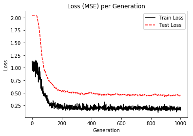
In [15]:
%matplotlib inline
# Plot loss (MSE) over time
plt.plot(train_loss, 'k-', label='Train Loss')
plt.plot(test_loss, 'r--', label='Test Loss')
plt.title('Loss (MSE) per Generation')
plt.legend(loc='upper right')
plt.xlabel('Generation')
plt.ylabel('Loss')
plt.show()

Tensorboard Graph
What follows is the graph we have executed and all data about it.

Predict
In [16]:
#
# Leave in blanck intentionally
#
We have reached the end of this post, but don’t worry, I will continue it very soon.
In the meantime, I propose that you put your infrastructure in place to create trading systems. Take a look at the following posts that are aimed at you acquiring good practices. So, your work could be reproducible.
Quant Trading Project Structure
Robust Git Workflow for Research Projects
Remember all these calculations are included in a Jupyter notebook in my Github repository:


1 COMMENT
[…] DeepTrading with TensorFlow III [Todo Trader] […]