 Black Belt
 Deep Trading with TensorFlow V
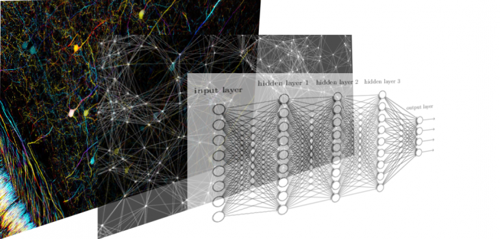
Do you want to know how to build a multi-layered neural network? As deep as you want?
In the next post, we will use real market data. In this one, we will still use non-trading data, because we are looking for a well-established knowledge of the basic concepts of Tensorflow. But we will use data used in other very real and current problems.
OK, remember to keep in mind our other posts that make up a systematic and complete structure to deal with problems of supervised machine learning:
https://todotrader.com/deeptrading-with-tensorflow/
https://todotrader.com/deeptrading-with-tensorflow-I/
https://todotrader.com/deeptrading-with-tensorflow-II/
https://todotrader.com/deeptrading-with-tensorflow-III/
https://todotrader.com/deeptrading-with-tensorflow-IV/
Implementing a multiple hidden layer Neural Network
The progress of the model can be saved during and after training. This means that a model can be resumed where it left off and avoid long training times. Saving also means that you can share your model and others can recreate your work.
In the last post, we presented a simple regression problem that we solved with a neural network with a single hidden layer. I made a prediction of one of the variables involved.
This type of prediction is called “problems or regression analysis”, compared to other types of problems such as “classification” (see Artifical Intelligence Taxonomy in my post, https://todotrader.com/artificial-intelligence-trading-systems /)
Regression analysis can help us to model the relationship between a dependent variable (which we are trying to predict) and one or more independent variables (the input of the model). The regression analysis can show if there is a significant relationship between the independent variables and the dependent variable, and the importance of their interrelation: when the independent variables move, how much can we expect the dependent variable to move?
We will illustrate how to create a multiple fully connected hidden layer NN, save it and make predictions with a
We will use a more complex data than the iris data is for this exercise. That dataset is “Concrete Compressive Strength Data Set” from https://archive.ics.uci.edu/ml/datasets/Concrete+Compressive+Strength
Data Characteristics:
The actual concrete compressive strength (MPa) for a given mixture under a specific age (days) was determined from laboratory. Data is in raw form (not scaled).
Summary Statistics:
Number of instances (observations): 1030 Number of Attributes: 9 Attribute breakdown: 8 quantitative input variables, and 1 quantitative output variable Missing Attribute Values: None
We will build a three-hidden layer neural network to predict the nineth attribute, the concrete compressive strength, from the other eight.
Load configuration
In [1]:
import seaborn as sns
import matplotlib.pyplot as plt
import numpy as np
import tensorflow as tf
#from sklearn.datasets import load_iris
from tensorflow.python.framework import ops
import pandas as pd
/home/parrondo/anaconda3/envs/deeptrading/lib/python3.5/importlib/_bootstrap.py:222: RuntimeWarning: numpy.dtype size changed, may indicate binary incompatibility. Expected 96, got 88
  return f(*args, **kwds)
/home/parrondo/anaconda3/envs/deeptrading/lib/python3.5/importlib/_bootstrap.py:222: RuntimeWarning: numpy.dtype size changed, may indicate binary incompatibility. Expected 96, got 88
  return f(*args, **kwds)
/home/parrondo/anaconda3/envs/deeptrading/lib/python3.5/importlib/_bootstrap.py:222: RuntimeWarning: numpy.dtype size changed, may indicate binary incompatibility. Expected 96, got 88
  return f(*args, **kwds)
Ingest raw data
In [2]:
# Dataset "Concrete Compressive Strength Data Set" from: https://archive.ics.uci.edu/ml/datasets/Concrete+Compressive+Strength
df = pd.read_excel(r'../data/raw/Concrete_Data.xls') #for an earlier version of Excel, you may need to use the file extension of 'xls'

#Simplifying column names
df.columns = ["Cement", "Blast Furnace Slag", "Fly Ash", "Water", "Superplasticizer",
              "Coarse Aggregate", "Fine Aggregate", "Age", "Strength"]
# We get a pandas dataframe to better visualize the datasets
df
Out[2]:
| Cement | Blast Furnace Slag | Fly Ash | Water | Superplasticizer | Coarse Aggregate | Fine Aggregate | Age | Strength | |
|---|---|---|---|---|---|---|---|---|---|
| 0 | 540.0 | 0.0 | 0.0 | 162.0 | 2.5 | 1040.0 | 676.0 | 28 | 79.986111 |
| 1 | 540.0 | 0.0 | 0.0 | 162.0 | 2.5 | 1055.0 | 676.0 | 28 | 61.887366 |
| 2 | 332.5 | 142.5 | 0.0 | 228.0 | 0.0 | 932.0 | 594.0 | 270 | 40.269535 |
| 3 | 332.5 | 142.5 | 0.0 | 228.0 | 0.0 | 932.0 | 594.0 | 365 | 41.052780 |
| 4 | 198.6 | 132.4 | 0.0 | 192.0 | 0.0 | 978.4 | 825.5 | 360 | 44.296075 |
| 5 | 266.0 | 114.0 | 0.0 | 228.0 | 0.0 | 932.0 | 670.0 | 90 | 47.029847 |
| 6 | 380.0 | 95.0 | 0.0 | 228.0 | 0.0 | 932.0 | 594.0 | 365 | 43.698299 |
| 7 | 380.0 | 95.0 | 0.0 | 228.0 | 0.0 | 932.0 | 594.0 | 28 | 36.447770 |
| 8 | 266.0 | 114.0 | 0.0 | 228.0 | 0.0 | 932.0 | 670.0 | 28 | 45.854291 |
| 9 | 475.0 | 0.0 | 0.0 | 228.0 | 0.0 | 932.0 | 594.0 | 28 | 39.289790 |
| 10 | 198.6 | 132.4 | 0.0 | 192.0 | 0.0 | 978.4 | 825.5 | 90 | 38.074244 |
| 11 | 198.6 | 132.4 | 0.0 | 192.0 | 0.0 | 978.4 | 825.5 | 28 | 28.021684 |
| 12 | 427.5 | 47.5 | 0.0 | 228.0 | 0.0 | 932.0 | 594.0 | 270 | 43.012960 |
| 13 | 190.0 | 190.0 | 0.0 | 228.0 | 0.0 | 932.0 | 670.0 | 90 | 42.326932 |
| 14 | 304.0 | 76.0 | 0.0 | 228.0 | 0.0 | 932.0 | 670.0 | 28 | 47.813782 |
| 15 | 380.0 | 0.0 | 0.0 | 228.0 | 0.0 | 932.0 | 670.0 | 90 | 52.908320 |
| 16 | 139.6 | 209.4 | 0.0 | 192.0 | 0.0 | 1047.0 | 806.9 | 90 | 39.358048 |
| 17 | 342.0 | 38.0 | 0.0 | 228.0 | 0.0 | 932.0 | 670.0 | 365 | 56.141962 |
| 18 | 380.0 | 95.0 | 0.0 | 228.0 | 0.0 | 932.0 | 594.0 | 90 | 40.563252 |
| 19 | 475.0 | 0.0 | 0.0 | 228.0 | 0.0 | 932.0 | 594.0 | 180 | 42.620648 |
| 20 | 427.5 | 47.5 | 0.0 | 228.0 | 0.0 | 932.0 | 594.0 | 180 | 41.836714 |
| 21 | 139.6 | 209.4 | 0.0 | 192.0 | 0.0 | 1047.0 | 806.9 | 28 | 28.237490 |
| 22 | 139.6 | 209.4 | 0.0 | 192.0 | 0.0 | 1047.0 | 806.9 | 3 | 8.063422 |
| 23 | 139.6 | 209.4 | 0.0 | 192.0 | 0.0 | 1047.0 | 806.9 | 180 | 44.207822 |
| 24 | 380.0 | 0.0 | 0.0 | 228.0 | 0.0 | 932.0 | 670.0 | 365 | 52.516697 |
| 25 | 380.0 | 0.0 | 0.0 | 228.0 | 0.0 | 932.0 | 670.0 | 270 | 53.300632 |
| 26 | 380.0 | 95.0 | 0.0 | 228.0 | 0.0 | 932.0 | 594.0 | 270 | 41.151375 |
| 27 | 342.0 | 38.0 | 0.0 | 228.0 | 0.0 | 932.0 | 670.0 | 180 | 52.124386 |
| 28 | 427.5 | 47.5 | 0.0 | 228.0 | 0.0 | 932.0 | 594.0 | 28 | 37.427515 |
| 29 | 475.0 | 0.0 | 0.0 | 228.0 | 0.0 | 932.0 | 594.0 | 7 | 38.603761 |
| … | … | … | … | … | … | … | … | … | … |
| 1000 | 141.9 | 166.6 | 129.7 | 173.5 | 10.9 | 882.6 | 785.3 | 28 | 44.611855 |
| 1001 | 297.8 | 137.2 | 106.9 | 201.3 | 6.0 | 878.4 | 655.3 | 28 | 53.524711 |
| 1002 | 321.3 | 164.2 | 0.0 | 190.5 | 4.6 | 870.0 | 774.0 | 28 | 57.218234 |
| 1003 | 366.0 | 187.0 | 0.0 | 191.3 | 6.6 | 824.3 | 756.9 | 28 | 65.909079 |
| 1004 | 279.8 | 128.9 | 100.4 | 172.4 | 9.5 | 825.1 | 804.9 | 28 | 52.826962 |
| 1005 | 252.1 | 97.1 | 75.6 | 193.8 | 8.3 | 835.5 | 821.4 | 28 | 33.399596 |
| 1006 | 164.6 | 0.0 | 150.4 | 181.6 | 11.7 | 1023.3 | 728.9 | 28 | 18.033934 |
| 1007 | 155.6 | 243.5 | 0.0 | 180.3 | 10.7 | 1022.0 | 697.7 | 28 | 37.363394 |
| 1008 | 160.2 | 188.0 | 146.4 | 203.2 | 11.3 | 828.7 | 709.7 | 28 | 35.314271 |
| 1009 | 298.1 | 0.0 | 107.0 | 186.4 | 6.1 | 879.0 | 815.2 | 28 | 42.644091 |
| 1010 | 317.9 | 0.0 | 126.5 | 209.7 | 5.7 | 860.5 | 736.6 | 28 | 40.062003 |
| 1011 | 287.3 | 120.5 | 93.9 | 187.6 | 9.2 | 904.4 | 695.9 | 28 | 43.798273 |
| 1012 | 325.6 | 166.4 | 0.0 | 174.0 | 8.9 | 881.6 | 790.0 | 28 | 61.235811 |
| 1013 | 355.9 | 0.0 | 141.6 | 193.3 | 11.0 | 801.4 | 778.4 | 28 | 40.868690 |
| 1014 | 132.0 | 206.5 | 160.9 | 178.9 | 5.5 | 866.9 | 735.6 | 28 | 33.306517 |
| 1015 | 322.5 | 148.6 | 0.0 | 185.8 | 8.5 | 951.0 | 709.5 | 28 | 52.426376 |
| 1016 | 164.2 | 0.0 | 200.1 | 181.2 | 12.6 | 849.3 | 846.0 | 28 | 15.091251 |
| 1017 | 313.8 | 0.0 | 112.6 | 169.9 | 10.1 | 925.3 | 782.9 | 28 | 38.461040 |
| 1018 | 321.4 | 0.0 | 127.9 | 182.5 | 11.5 | 870.1 | 779.7 | 28 | 37.265488 |
| 1019 | 139.7 | 163.9 | 127.7 | 236.7 | 5.8 | 868.6 | 655.6 | 28 | 35.225329 |
| 1020 | 288.4 | 121.0 | 0.0 | 177.4 | 7.0 | 907.9 | 829.5 | 28 | 42.140084 |
| 1021 | 298.2 | 0.0 | 107.0 | 209.7 | 11.1 | 879.6 | 744.2 | 28 | 31.875165 |
| 1022 | 264.5 | 111.0 | 86.5 | 195.5 | 5.9 | 832.6 | 790.4 | 28 | 41.542308 |
| 1023 | 159.8 | 250.0 | 0.0 | 168.4 | 12.2 | 1049.3 | 688.2 | 28 | 39.455954 |
| 1024 | 166.0 | 259.7 | 0.0 | 183.2 | 12.7 | 858.8 | 826.8 | 28 | 37.917043 |
| 1025 | 276.4 | 116.0 | 90.3 | 179.6 | 8.9 | 870.1 | 768.3 | 28 | 44.284354 |
| 1026 | 322.2 | 0.0 | 115.6 | 196.0 | 10.4 | 817.9 | 813.4 | 28 | 31.178794 |
| 1027 | 148.5 | 139.4 | 108.6 | 192.7 | 6.1 | 892.4 | 780.0 | 28 | 23.696601 |
| 1028 | 159.1 | 186.7 | 0.0 | 175.6 | 11.3 | 989.6 | 788.9 | 28 | 32.768036 |
| 1029 | 260.9 | 100.5 | 78.3 | 200.6 | 8.6 | 864.5 | 761.5 | 28 | 32.401235 |
1030 rows × 9 columns
In [3]:
# Now our usual X, y variables
X_raw = df[df.columns[0:8]].values
y_raw = df[df.columns[8]].values

# Dimensions of dataset
print("Dimensions of dataset")
n = X_raw.shape[0]
p = X_raw.shape[1]
print("n=",n,"p=",p)
Dimensions of dataset
n= 1030 p= 8
In [4]:
X_raw.shape # Array 1030x8. Each element is an 8-dimensional data point: Cement, Blast Furnace Slag, Fly Ash,…
Out[4]:
(1030, 8)In [5]:
y_raw.shape Vector 1030. Each element is a 1-dimensional (scalar) data point: Strength
Out[5]:
(1030,)In [6]:
# We can confirm the data are right with a simple visualization.
X_raw
Out[6]:
array([[ 540. ,    0. ,    0. , ..., 1040. ,  676. ,   28. ],
       [ 540. ,    0. ,    0. , ..., 1055. ,  676. ,   28. ],
       [ 332.5,  142.5,    0. , ...,  932. ,  594. ,  270. ],
       ...,
       [ 148.5,  139.4,  108.6, ...,  892.4,  780. ,   28. ],
       [ 159.1,  186.7,    0. , ...,  989.6,  788.9,   28. ],
       [ 260.9,  100.5,   78.3, ...,  864.5,  761.5,   28. ]])
In [7]:
y_raw
Out[7]:
array([79.98611076, 61.88736576, 40.26953526, ..., 23.69660064,
       32.76803638, 32.40123514])
Basic pre-process data
Checking multicollinearity of pairs
Plotting the pairwise scatterplots
Pairwise scatter plots and correlation heatmap are usual visual tools for checking multicollinearity. We can use the pairplot function from the seaborn library to plot the pairwise scatterplots of all combinations.
In [8]:
# Visualization
sns.set_style("whitegrid");
sns.pairplot(df);
plt.show()

As you can see it is a pretty difficult problem. There are almost no correlations between Strenght and the other features. Visually we can see some correlation of Strenght with the kind of Cement (it is not surprising, of course).
Plotting a diagonal correlation matrix
Now we are going to plot the diagonal correlation matrix with Seaborn:
In [9]:
# Correlation
sns.set(style="white")

# Generate a large random dataset
rs = np.random.RandomState(33)

# Compute the correlation matrix
corr = df.corr()

# Generate a mask for the upper triangle
mask = np.zeros_like(corr, dtype=np.bool)
mask[np.triu_indices_from(mask)] = True

# Set up the matplotlib figure
f, ax = plt.subplots(figsize=(11, 9))

# Generate a custom diverging colormap
cmap = sns.diverging_palette(220, 10, as_cmap=True)

# Draw the heatmap with the mask and correct aspect ratio
sns.heatmap(corr, mask=mask, cmap=cmap, vmax=.3, center=0,
            square=True, linewidths=.5, cbar_kws={"shrink": .5})
Out[9]:
<matplotlib.axes._subplots.AxesSubplot at 0x7ff0696ddb38>

In [10]:
#
# We could try to make some pre-processing of data in order to find or simplify features,
# but it is a problem for another notebook. Now we mantain the focus on the basis.
#
Split data
In [11]:
# split into train and test sets

# Total samples
nsamples = n

# Splitting into train (90%) and test (10%) sets
split = 90 # training split% ; test (100-split)%
jindex = nsamples*split//100 # Index for slicing the samples

# Samples in train
nsamples_train = jindex

# Samples in test
nsamples_test = nsamples - nsamples_train
print("Total number of samples: ",nsamples,"\nSamples in train set: ", nsamples_train,
      "\nSamples in test set: ",nsamples_test)

# Here are train and test samples
X_train = X_raw[:jindex, :]
y_train = y_raw[:jindex]

X_test = X_raw[jindex:, :]
y_test = y_raw[jindex:]

print("X_train.shape = ", X_train.shape, "y_train.shape =", y_train.shape, "\nX_test.shape =  ",
      X_test.shape, "y_test.shape = ", y_test.shape)
Total number of samples:  1030
Samples in train set:  927
Samples in test set:  103
X_train.shape =  (927, 8) y_train.shape = (927,)
X_test.shape =   (103, 8) y_test.shape =  (103,)
Transform features
Note
Be careful not to write X_test_std = sc.fit_transform(X_test) instead of X_test_std = sc.transform(X_test). In this case, it wouldn’t make a great difference since the mean and standard deviation of the test set should be (quite) similar to the training set. However, this is not always the case in Forex market data, as has been well established in the literature. The correct way is to re-use parameters from the training set if we are doing any kind of transformation. So, the test set should basically stand for “new, unseen” data. In [12]:
# Scale data
from sklearn.preprocessing import StandardScaler

sc = StandardScaler()
X_train_std = sc.fit_transform(X_train)
X_test_std = sc.transform(X_test)

y_train_std = sc.fit_transform(y_train.reshape(-1, 1))
y_test_std = sc.transform(y_test.reshape(-1, 1))
/home/parrondo/anaconda3/envs/deeptrading/lib/python3.5/importlib/_bootstrap.py:222: RuntimeWarning: numpy.dtype size changed, may indicate binary incompatibility. Expected 96, got 88
  return f(*args, **kwds)
/home/parrondo/anaconda3/envs/deeptrading/lib/python3.5/importlib/_bootstrap.py:222: RuntimeWarning: numpy.dtype size changed, may indicate binary incompatibility. Expected 96, got 88
  return f(*args, **kwds)
In [13]:
y_test
Out[13]:
array([33.05347944, 24.5798194 , 21.91154728, 30.88163004, 15.340841  ,
       24.3385028 , 23.8903434 , 22.93197176, 29.41304616, 28.62980142,
       36.80491836, 18.28766142, 32.72046253, 31.4201108 , 28.9379972 ,
       40.92522693, 12.18097249, 25.5595648 , 36.44363293, 32.96384756,
       23.8358748 , 26.23318285, 17.95947085, 38.6306508 , 19.0095428 ,
       33.71882378,  8.53640236, 13.46132942, 32.24541357, 23.52423164,
       29.72606826, 49.77327244, 52.44637089, 40.9348796 , 44.86834018,
       13.20208645, 37.43165204, 29.87085822, 56.61907964, 12.4595208 ,
       23.786922  , 13.29378676, 39.42147978, 46.23419213, 44.52360218,
       23.74417449, 26.14768782, 15.52631004, 43.57833058, 35.86585204,
       41.05346947, 28.99108685, 46.24729218, 26.92265885, 10.53588276,
       25.10382116, 29.07313449,  9.73815902, 33.798803  , 37.17103011,
       33.76226077, 16.50398701, 19.98790924, 36.3498642 , 38.21558625,
       15.42357812, 33.4195912 , 39.0560575 , 27.68108245, 26.85991653,
       45.30477848, 30.12320644, 15.56974703, 44.6118551 , 53.52471136,
       57.21823429, 65.90907927, 52.82696164, 33.39959639, 18.03393426,
       37.36339392, 35.31427124, 42.6440906 , 40.06200298, 43.79827342,
       61.23581094, 40.8686899 , 33.30651713, 52.42637609, 15.09125069,
       38.46103971, 37.26548832, 35.22532884, 42.14008364, 31.87516496,
       41.54230795, 39.45595358, 37.91704314, 44.284354  , 31.1787942 ,
       23.69660064, 32.76803638, 32.40123514])
But we can revert the situation if we need.
In [14]:
sc.inverse_transform(y_test_std)
Out[14]:
array([[33.05347944],
       [24.5798194 ],
       [21.91154728],
       [30.88163004],
       [15.340841  ],
       [24.3385028 ],
       [23.8903434 ],
       [22.93197176],
       [29.41304616],
       [28.62980142],
       [36.80491836],
       [18.28766142],
       [32.72046253],
       [31.4201108 ],
       [28.9379972 ],
       [40.92522693],
       [12.18097249],
       [25.5595648 ],
       [36.44363293],
       [32.96384756],
       [23.8358748 ],
       [26.23318285],
       [17.95947085],
       [38.6306508 ],
       [19.0095428 ],
       [33.71882378],
       [ 8.53640236],
       [13.46132942],
       [32.24541357],
       [23.52423164],
       [29.72606826],
       [49.77327244],
       [52.44637089],
       [40.9348796 ],
       [44.86834018],
       [13.20208645],
       [37.43165204],
       [29.87085822],
       [56.61907964],
       [12.4595208 ],
       [23.786922  ],
       [13.29378676],
       [39.42147978],
       [46.23419213],
       [44.52360218],
       [23.74417449],
       [26.14768782],
       [15.52631004],
       [43.57833058],
       [35.86585204],
       [41.05346947],
       [28.99108685],
       [46.24729218],
       [26.92265885],
       [10.53588276],
       [25.10382116],
       [29.07313449],
       [ 9.73815902],
       [33.798803  ],
       [37.17103011],
       [33.76226077],
       [16.50398701],
       [19.98790924],
       [36.3498642 ],
       [38.21558625],
       [15.42357812],
       [33.4195912 ],
       [39.0560575 ],
       [27.68108245],
       [26.85991653],
       [45.30477848],
       [30.12320644],
       [15.56974703],
       [44.6118551 ],
       [53.52471136],
       [57.21823429],
       [65.90907927],
       [52.82696164],
       [33.39959639],
       [18.03393426],
       [37.36339392],
       [35.31427124],
       [42.6440906 ],
       [40.06200298],
       [43.79827342],
       [61.23581094],
       [40.8686899 ],
       [33.30651713],
       [52.42637609],
       [15.09125069],
       [38.46103971],
       [37.26548832],
       [35.22532884],
       [42.14008364],
       [31.87516496],
       [41.54230795],
       [39.45595358],
       [37.91704314],
       [44.284354  ],
       [31.1787942 ],
       [23.69660064],
       [32.76803638],
       [32.40123514]])
Implement the model
In [15]:
# Clears the default graph stack and resets the global default graph
ops.reset_default_graph()
In [16]:
# make results reproducible
seed = 2
tf.set_random_seed(seed)
np.random.seed(seed)


# Parameters
learning_rate = 0.005
batch_size = 50
n_features = X_train.shape[1]#  Number of features in training data
epochs = 10000
display_step = 100
model_path = "../model/tmp/model.ckpt"
n_classes = 1

# Network Parameters
# See figure of the model
d0 = D = n_features # Layer 0 (Input layer number of features)
d1 = 5 # Layer 1 (5 hidden nodes)
d2 = 15 # Layer 2 (15 hidden nodes)
d3 = 5 # Layer 3 (5 hidden nodes)
d4 = C = 1 # Layer 4 (Output layer)

# tf Graph input
print("Placeholders")
X = tf.placeholder(dtype=tf.float32, shape=[None, n_features], name="X")
y = tf.placeholder(dtype=tf.float32, shape=[None,n_classes], name="y")


# Initializers
print("Initializers")
sigma = 1
weight_initializer = tf.variance_scaling_initializer(mode="fan_avg", distribution="uniform", scale=sigma)
bias_initializer = tf.zeros_initializer()

# Create model
def multilayer_perceptron(X, variables):
    # Hidden layer with ReLU activation
    layer_1 = tf.nn.relu(tf.add(tf.matmul(X, variables['W1']), variables['bias1']))
    # Hidden layer with ReLU activation
    layer_2 = tf.nn.relu(tf.add(tf.matmul(layer_1, variables['W2']), variables['bias2']))
    # Hidden layer with ReLU activation
    layer_3 = tf.nn.relu(tf.add(tf.matmul(layer_2, variables['W3']), variables['bias3']))
    # Output layer with ReLU activation
    out_layer = tf.nn.relu(tf.add(tf.matmul(layer_3, variables['W4']), variables['bias4']))
    return out_layer

# Store layers weight & bias
variables = {
    'W1': tf.Variable(weight_initializer([n_features, d1]), name="W1"), # inputs -> d1 hidden neurons
    'bias1': tf.Variable(bias_initializer([d1]), name="bias1"), # one biases for each d1 hidden neurons
    'W2': tf.Variable(weight_initializer([d1, d2]), name="W2"), # d1 hidden inputs -> d2 hidden neurons
    'bias2': tf.Variable(bias_initializer([d2]), name="bias2"), # one biases for each d2 hidden neurons
    'W3': tf.Variable(weight_initializer([d2, d3]), name="W3"), ## d2 hidden inputs -> d3 hidden neurons
    'bias3': tf.Variable(bias_initializer([d3]), name="bias3"), # one biases for each d3 hidden neurons
    'W4': tf.Variable(weight_initializer([d3, d4]), name="W4"), # d3 hidden inputs -> 1 output
    'bias4': tf.Variable(bias_initializer([d4]), name="bias4") # 1 bias for the output
}

# Construct model
y_hat = multilayer_perceptron(X, variables)

# Define loss and optimizer
loss = tf.reduce_mean(tf.square(y - y_hat)) # MSE
optimizer = tf.train.GradientDescentOptimizer(learning_rate).minimize(loss) # Train step

# Initialize the variables (i.e. assign their default value)
init = tf.global_variables_initializer()

# 'Saver' op to save and restore all the variables
saver = tf.train.Saver()
Placeholders
Initializers
Train the model and Evaluate the model
In [17]:
# Running first session
print("Starting 1st session...")
with tf.Session() as sess:

    # Writer to record image, scalar, histogram and graph for display in tensorboard
    writer = tf.summary.FileWriter("../model/tmp/tensorflow_logs", sess.graph)  # create writer
    writer.add_graph(sess.graph)

    # Run the initializer
    sess.run(init)

    # Training cycle
    train_loss = []
    test_loss = []

    for epoch in range(epochs):
        rand_index = np.random.choice(len(X_train_std), size=batch_size)
        X_rand = X_train_std[rand_index]
        y_rand = y_train_std[rand_index]
        #y_rand = np.transpose([y_train[rand_index]])
        sess.run(optimizer, feed_dict={X: X_rand, y: y_rand})

        train_temp_loss = sess.run(loss, feed_dict={X: X_rand, y: y_rand})
        train_loss.append(np.sqrt(train_temp_loss))

        test_temp_loss = sess.run(loss, feed_dict={X: X_test_std, y: y_test_std})
        #test_temp_loss = sess.run(loss, feed_dict={X: X_test_std, y: np.transpose([y_test])})
        test_loss.append(np.sqrt(test_temp_loss))
        if (epoch+1) % display_step == 0:
            print("Epoch:", '%04d' % (epoch+1), "Loss=", \
                "{:.9f}".format(train_temp_loss))

    # Close writer
    writer.flush()
    writer.close()

    # Save model weights to disk
    save_path = saver.save(sess, model_path)
    print("Model saved in file: %s" % save_path)
    print("First Optimization Finished!")
Starting 1st session...
Epoch: 0100 Loss= 1.187452793
Epoch: 0200 Loss= 0.653784931
Epoch: 0300 Loss= 0.850386798
Epoch: 0400 Loss= 0.666906953
Epoch: 0500 Loss= 0.922570705
Epoch: 0600 Loss= 0.788938463
Epoch: 0700 Loss= 0.720452368
Epoch: 0800 Loss= 0.650036752
Epoch: 0900 Loss= 0.696900964
Epoch: 1000 Loss= 0.559514642
Epoch: 1100 Loss= 0.576028287
Epoch: 1200 Loss= 0.649010479
Epoch: 1300 Loss= 0.679859638
Epoch: 1400 Loss= 0.513536632
Epoch: 1500 Loss= 0.522186100
Epoch: 1600 Loss= 0.464669585
Epoch: 1700 Loss= 0.482417375
Epoch: 1800 Loss= 0.514982164
Epoch: 1900 Loss= 0.873984993
Epoch: 2000 Loss= 0.710068643
Epoch: 2100 Loss= 0.583979726
Epoch: 2200 Loss= 0.510860145
Epoch: 2300 Loss= 0.409339219
Epoch: 2400 Loss= 0.689149320
Epoch: 2500 Loss= 0.465828985
Epoch: 2600 Loss= 0.475971222
Epoch: 2700 Loss= 0.609764397
Epoch: 2800 Loss= 0.535831273
Epoch: 2900 Loss= 0.499730915
Epoch: 3000 Loss= 0.495828092
Epoch: 3100 Loss= 0.536907375
Epoch: 3200 Loss= 0.523644745
Epoch: 3300 Loss= 0.694934130
Epoch: 3400 Loss= 0.761239827
Epoch: 3500 Loss= 0.659935832
Epoch: 3600 Loss= 0.594260037
Epoch: 3700 Loss= 0.426724046
Epoch: 3800 Loss= 0.568280101
Epoch: 3900 Loss= 0.541940570
Epoch: 4000 Loss= 0.557236254
Epoch: 4100 Loss= 0.574568808
Epoch: 4200 Loss= 0.530215859
Epoch: 4300 Loss= 0.757081807
Epoch: 4400 Loss= 0.486846477
Epoch: 4500 Loss= 0.601066351
Epoch: 4600 Loss= 0.541417539
Epoch: 4700 Loss= 0.496193975
Epoch: 4800 Loss= 0.665046215
Epoch: 4900 Loss= 0.676892161
Epoch: 5000 Loss= 0.389218241
Epoch: 5100 Loss= 0.538830817
Epoch: 5200 Loss= 0.345810086
Epoch: 5300 Loss= 0.470290005
Epoch: 5400 Loss= 0.720839977
Epoch: 5500 Loss= 0.593623638
Epoch: 5600 Loss= 0.359151542
Epoch: 5700 Loss= 0.415069729
Epoch: 5800 Loss= 0.525559127
Epoch: 5900 Loss= 0.364094764
Epoch: 6000 Loss= 0.461983174
Epoch: 6100 Loss= 0.440127134
Epoch: 6200 Loss= 0.368957520
Epoch: 6300 Loss= 0.528110206
Epoch: 6400 Loss= 0.443941981
Epoch: 6500 Loss= 0.693621516
Epoch: 6600 Loss= 0.591214240
Epoch: 6700 Loss= 0.628453016
Epoch: 6800 Loss= 0.600034475
Epoch: 6900 Loss= 0.474740833
Epoch: 7000 Loss= 0.448413581
Epoch: 7100 Loss= 0.407264739
Epoch: 7200 Loss= 0.508368433
Epoch: 7300 Loss= 0.560470521
Epoch: 7400 Loss= 0.457139134
Epoch: 7500 Loss= 0.415577382
Epoch: 7600 Loss= 0.366004378
Epoch: 7700 Loss= 0.743126690
Epoch: 7800 Loss= 0.570745826
Epoch: 7900 Loss= 0.420384288
Epoch: 8000 Loss= 0.515913427
Epoch: 8100 Loss= 0.345190585
Epoch: 8200 Loss= 0.593500078
Epoch: 8300 Loss= 0.634471953
Epoch: 8400 Loss= 0.403643250
Epoch: 8500 Loss= 0.410774380
Epoch: 8600 Loss= 0.522914648
Epoch: 8700 Loss= 0.450753480
Epoch: 8800 Loss= 0.415820956
Epoch: 8900 Loss= 0.760270894
Epoch: 9000 Loss= 0.478740126
Epoch: 9100 Loss= 0.467870414
Epoch: 9200 Loss= 0.568970919
Epoch: 9300 Loss= 0.707495451
Epoch: 9400 Loss= 0.528955817
Epoch: 9500 Loss= 0.630569756
Epoch: 9600 Loss= 0.737566054
Epoch: 9700 Loss= 0.482343763
Epoch: 9800 Loss= 0.543290317
Epoch: 9900 Loss= 0.706319273
Epoch: 10000 Loss= 0.350363821
Model saved in file: ../model/tmp/model.ckpt
First Optimization Finished!
In [18]:
%matplotlib inline
# Plot loss (MSE) over time
plt.plot(train_loss[100:], 'k-', label='Train Loss')
plt.plot(test_loss[100:], 'r--', label='Test Loss')
plt.title('Loss (MSE) per Generation')
plt.legend(loc='upper right')
plt.xlabel('Generation')
plt.ylabel('Loss')
plt.show()

We can see the error of this model is big. So, it is not a very accurate model.
Tensorboard Graph
What follows is the graph we have executed and all data about it. Note the “save” label and the several layers.

Saving a TensorFlow model
So, now we have our model saved.
Tensorflow model has four main files:
- a) Meta graph: This is a protocol buffer which saves the complete Tensorflow graph; i.e. all variables, operations, collections etc. This file has .meta extension.
- b) y c) Checkpoint files: It is a binary file which contains all the values of the weights, biases, gradients and all the other variables saved. Tensorflow has changed from version 0.11. Instead of a single .ckpt file, we have now two files: .index and .data file that contains our training variables.
- d) Along with this, Tensorflow also has a file named checkpoint which simply keeps a record of latest checkpoint files saved.
Retrain the model
We can retrain the model as many times as we want to. In [19]:
# Running a new session
print("Starting 2nd session...")
with tf.Session() as sess:
    # Initialize variables
    sess.run(init)

    # Restore model weights from previously saved model
    saver.restore(sess, model_path)
    print("Model restored from file: %s" % model_path)

    # Resume training
    for epoch in range(epochs):
        rand_index = np.random.choice(len(X_train), size=batch_size)
        X_rand = X_train_std[rand_index]
        y_rand = y_train_std[rand_index]
        #y_rand = np.transpose([y_train[rand_index]])
        sess.run(optimizer, feed_dict={X: X_rand, y: y_rand})

        train_temp_loss = sess.run(loss, feed_dict={X: X_rand, y: y_rand})
        train_loss.append(np.sqrt(train_temp_loss))

        test_temp_loss = sess.run(loss, feed_dict={X: X_test_std, y: y_test_std})
        # test_temp_loss = sess.run(loss, feed_dict={X: X_test_std, y: np.transpose([y_test])})
        test_loss.append(np.sqrt(test_temp_loss))
        if (epoch+1) % display_step == 0:
            print("Epoch:", '%04d' % (epoch+1), "Loss=", \
                "{:.9f}".format(train_temp_loss))

    # Close writer
    writer.flush()
    writer.close()

    # Save model weights to disk
    save_path = saver.save(sess, model_path)
    print("Model saved in file: %s" % save_path)
    print("Second Optimization Finished!")
Starting 2nd session...
INFO:tensorflow:Restoring parameters from ../model/tmp/model.ckpt
Model restored from file: ../model/tmp/model.ckpt
Epoch: 0100 Loss= 0.553170979
Epoch: 0200 Loss= 0.394454986
Epoch: 0300 Loss= 0.430046231
Epoch: 0400 Loss= 0.474143565
Epoch: 0500 Loss= 0.581448019
Epoch: 0600 Loss= 0.509629428
Epoch: 0700 Loss= 0.395796895
Epoch: 0800 Loss= 0.555636227
Epoch: 0900 Loss= 0.343794316
Epoch: 1000 Loss= 0.837739229
Epoch: 1100 Loss= 0.313927382
Epoch: 1200 Loss= 0.527575970
Epoch: 1300 Loss= 0.503197849
Epoch: 1400 Loss= 0.409355879
Epoch: 1500 Loss= 0.603905439
Epoch: 1600 Loss= 0.409259796
Epoch: 1700 Loss= 0.363913029
Epoch: 1800 Loss= 0.405373842
Epoch: 1900 Loss= 0.355158567
Epoch: 2000 Loss= 0.567333281
Epoch: 2100 Loss= 0.626644850
Epoch: 2200 Loss= 0.366723627
Epoch: 2300 Loss= 0.392675012
Epoch: 2400 Loss= 0.459658206
Epoch: 2500 Loss= 0.624418736
Epoch: 2600 Loss= 0.503614545
Epoch: 2700 Loss= 0.536920547
Epoch: 2800 Loss= 0.298828572
Epoch: 2900 Loss= 0.674796045
Epoch: 3000 Loss= 0.548250556
Epoch: 3100 Loss= 0.545930266
Epoch: 3200 Loss= 0.614865839
Epoch: 3300 Loss= 0.528206229
Epoch: 3400 Loss= 0.464911759
Epoch: 3500 Loss= 0.575236857
Epoch: 3600 Loss= 0.532283604
Epoch: 3700 Loss= 0.456996202
Epoch: 3800 Loss= 0.412953496
Epoch: 3900 Loss= 0.472213984
Epoch: 4000 Loss= 0.478306949
Epoch: 4100 Loss= 0.585611463
Epoch: 4200 Loss= 0.535116374
Epoch: 4300 Loss= 0.439250022
Epoch: 4400 Loss= 0.394633591
Epoch: 4500 Loss= 0.543169975
Epoch: 4600 Loss= 0.678306758
Epoch: 4700 Loss= 0.401767313
Epoch: 4800 Loss= 0.717293620
Epoch: 4900 Loss= 0.395379066
Epoch: 5000 Loss= 0.619805276
Epoch: 5100 Loss= 0.558279872
Epoch: 5200 Loss= 0.435946107
Epoch: 5300 Loss= 0.512710631
Epoch: 5400 Loss= 0.596122563
Epoch: 5500 Loss= 0.624202967
Epoch: 5600 Loss= 0.406295478
Epoch: 5700 Loss= 0.477687240
Epoch: 5800 Loss= 0.500929236
Epoch: 5900 Loss= 0.388294727
Epoch: 6000 Loss= 0.515086234
Epoch: 6100 Loss= 0.513015807
Epoch: 6200 Loss= 0.541478157
Epoch: 6300 Loss= 0.551055014
Epoch: 6400 Loss= 0.320969999
Epoch: 6500 Loss= 0.418038338
Epoch: 6600 Loss= 0.324854702
Epoch: 6700 Loss= 0.482309490
Epoch: 6800 Loss= 0.451527864
Epoch: 6900 Loss= 0.578172445
Epoch: 7000 Loss= 0.441889644
Epoch: 7100 Loss= 0.649310470
Epoch: 7200 Loss= 0.584093750
Epoch: 7300 Loss= 0.546306133
Epoch: 7400 Loss= 0.403149009
Epoch: 7500 Loss= 0.547944903
Epoch: 7600 Loss= 0.494749665
Epoch: 7700 Loss= 0.388097167
Epoch: 7800 Loss= 0.602027893
Epoch: 7900 Loss= 0.430499852
Epoch: 8000 Loss= 0.684577465
Epoch: 8100 Loss= 0.413421541
Epoch: 8200 Loss= 0.450443357
Epoch: 8300 Loss= 0.311192632
Epoch: 8400 Loss= 0.642973185
Epoch: 8500 Loss= 0.478902638
Epoch: 8600 Loss= 0.665206373
Epoch: 8700 Loss= 0.606129229
Epoch: 8800 Loss= 0.493207961
Epoch: 8900 Loss= 0.620301306
Epoch: 9000 Loss= 0.489933938
Epoch: 9100 Loss= 0.447370619
Epoch: 9200 Loss= 0.593291521
Epoch: 9300 Loss= 0.488727689
Epoch: 9400 Loss= 0.468365222
Epoch: 9500 Loss= 0.465868115
Epoch: 9600 Loss= 0.548444033
Epoch: 9700 Loss= 0.501695275
Epoch: 9800 Loss= 0.455697834
Epoch: 9900 Loss= 0.423523307
Epoch: 10000 Loss= 0.724091947
Model saved in file: ../model/tmp/model.ckpt
Second Optimization Finished!
Predict
Finally, we can use the model to make some predictions. First
sc.transform([[203.5, 305.3, 0.0, 203.5, 0.0, 963.4, 630.0, 90],
              [173.0, 116.0, 0.0, 192.0, 0.0, 946.8, 856.8, 90],
              [522.0, 0.0, 0.0, 146.0, 0.0, 896.0, 896.0, 7]]) #True value  51.86, 32.10, 50.51
Out[20]:
array([[ 9.78564946, 15.74026644, -2.11773518,  9.78564946, -2.11773518,
        54.23470101, 34.73303791,  3.14666097],
       [ 8.00160409,  4.66748653, -2.11773518,  9.11297662, -2.11773518,
        53.26371238, 47.99931622,  3.14666097],
       [28.41576252, -2.11773518, -2.11773518,  6.42228525, -2.11773518,
        50.29225322, 50.29225322, -1.70828215]])
Then, we make the predictions:
In [21]:
# Running a new session for predictions
print("Starting prediction session...")
with tf.Session() as sess:
    # Initialize variables
    sess.run(init)

    # Restore model weights from previously saved model
    saver.restore(sess, model_path)
    print("Model restored from file: %s" % model_path)

    # We try to predict the Concrete compressive strength (MPa megapascals) of three samples
    feed_dict_std = {X: [[ 9.78564946, 15.74026644, -2.11773518,  9.78564946, -2.11773518,
        54.23470101, 34.73303791,  3.14666097],
       [ 8.00160409,  4.66748653, -2.11773518,  9.11297662, -2.11773518,
        53.26371238, 47.99931622,  3.14666097],
       [28.41576252, -2.11773518, -2.11773518,  6.42228525, -2.11773518,
        50.29225322, 50.29225322, -1.70828215]]}
    prediction = sess.run(y_hat, feed_dict_std)
    print(prediction) #True value  51.86, 32.10, 50.51
Starting prediction session...
INFO:tensorflow:Restoring parameters from ../model/tmp/model.ckpt
Model restored from file: ../model/tmp/model.ckpt
[[0.137997 ]
 [0.137997 ]
 [1.1572909]]
OK, better results, but still not very good results. We could try to improve them with a deeper network (more layers) or retouching the net parameters and number of neurons. That is another story.
In [22]:
y_hat_rev = sc.inverse_transform(prediction)
y_hat_rev
Out[22]:
array([[38.563946],
       [38.563946],
       [55.989773]], dtype=float32)
Not really good but illustrative of using deep neural network for this kind of difficult problems.
You can find the complete Jupyter notebooks (two notebooks because the second one is for restoring the model) in my Github repository:
https://github.com/parrondo/deeptrading
At last! In the next post Tensorflow with real data of financial markets. We will see how far we are able to arrive with this magnificent calculation and forecasting tool. 🙂
Meanwhile, I invite you to read my post about artificial intelligence applied to trading systems so that you have a bird’s eye view of the resources that we will be exploring in our series of articles.


3 COMMENTS
[…] Deep Trading with TensorFlow V [Todo Trader] […]
Hola,
felicidades por el blog y especialmente por esta serie de artículos sobre Tensorflow.
I am very interested on applying AI to trading and your blog is exactly what I was looking for. Until now, I have followed it reproducing what you have done. However I have a ton of doubts, specially in this last one.
1) My first questions is about number or neurons and layers. You have decide 3 hidden layers 5, 15, 5 neurons. But what would be the criteria to decide how many layers /neurons per layers fit the best to our problem? Number of combinations are almost infinite. How to decide if it is better more neurons or more layers?
2) In ML there are other type of algoritms (Polinomic regression, KNN, etc) how to know if for our problem (trading) NN is better than the others?
3) Why transformation and normalization are needed? Are we assuming that all input variables will have a gaussian distribution by doing this? if so, could it impact negatively in the final model? As we are applying the linear / non-linear steps to each attribute, the NN should deduce the right parameters even without normalizing the input variables.
4) why in each “epoch” you chose a subset of the data and not to run each one with the full training data? How the size of the “batch” could impact in the final result?
Gracias por compartir este conocimiento y hacerlo accesible a mas gente.
Saludos.
Hi JL,
Gracias por tus comentarios. Veo que hablas muy bien español.
I want to answer precisely all of your questions. However, I have to tell you that these exercises are just toys examples. Why? Because the purpose of the series is to serve as templates to place orders in our broker. And I want to do that as soon as possible. Once we have constructed a sound framework, then we can make all kind of changes in parameters, configuration, type of neural network, and so. So I only have used some unusual simple settings and arrangements which work, that’s all. All your questions are difficult to answer now, but we will explore all of them shortly.