OK, you know what tensors are or perhaps you don’t, but you are sure you want to use TensorFlow to trade with it. This post introduces you to how to create elemental NN tensors in TensorFlow.

This is the second post of the serie, so you need to be familiarized with the concepts exposed in the first post DeepTrading with Tensorflow.

Tensors

Tensors (of order higher than two) are data structures indexed by three or more indices, say (i,j,k,…) — a generalization of matrices, which are indexed by two indices, (m,n) for (m rows, n columns). These algebraic animals are very interesting from a theoretical point of view, and tensor-based methods have recently become very important in signal processing, data science, and machine learning applications.

Internally, TensorFlow represents tensors as n-dimensional arrays of base data types.

We use tensors all the time in Deep Learning, but you do not need to be an expert in them to use it. You may need to understand a little about them, so here are some good resources:

• Era of Big Data Processing: A New Approach via Tensor Networks and Tensor Decompositions
• Quick ML Concepts: Tensors
• Tensors: a tool for data science

How to create elemental NN tensors in TensorFlow

The following is an elemental computational graph that we are going to create and execute. It is very similar to many of the calculations that must be made in artificial neural networks. We will use Jupyter notebook to accomplish all calculations.

It is formed by a linear transformation, xW + b, followed by a non-linear activation fucntion, ReLU(). Where:

• x is a D-dimensional data point.
• W is the DxM matrix of weights.
• b is the bias M-dimensional vector

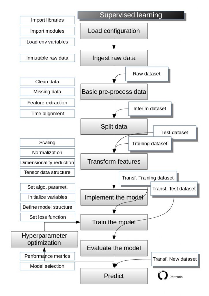
We will always follow the supervised flowchart:

Remember that you can find the complete Jupyter notebook in my Github repository:

https://github.com/parrondo/deeptrading

LOAD CONFIGURATION

First, we start with loading TensorFlow and resetting the computational graph.

In [1]:

import tensorflow as tf #Tensorflow 1.5 import warnings https://github.com/ContinuumIO/anaconda-issues/issues/6678
from tensorflow.python.framework import ops
ops.reset_default_graph()
import random as rnd
import numpy as np

/home/parrondo/anaconda3/envs/deeptrading/lib/python3.5/importlib/_bootstrap.py:222: RuntimeWarning: numpy.dtype size changed, may indicate binary incompatibility. Expected 96, got 88
  return f(*args, **kwds)
/home/parrondo/anaconda3/envs/deeptrading/lib/python3.5/importlib/_bootstrap.py:222: RuntimeWarning: numpy.dtype size changed, may indicate binary incompatibility. Expected 96, got 88
  return f(*args, **kwds)

IMPLEMENT THE MODEL

1. Build a graph

• a. Graph contains parameter specifications, model architecture, optimization process, …
• b. Somewhere between 5 and 5000 lines

These are the elements involved in our graph:

• Variables are 0-ary stateful nodes which output their current value.
• Placeholders are 0-ary nodes whose value is fed in at execution time.
• Mathematical operations:
  • MatMul: Multiply two matrix values.
  • Add: Add elementwise (with broadcasting).
  • ReLU: Activate with elementwise rectified linear function.

In [2]:

b = tf.Variable(tf.zeros((100,)), name='biases')
W=tf.Variable(tf.random_uniform((1024, 100), -1, 1), name='weights')
x = tf.placeholder(tf.float32, (1, 1024), name="x")
h_i = tf.nn.relu(tf.matmul(x, W) + b, name="h_i")

Now, you can see what the object b is:

In [3]:

b

And the output:

Out[3]:

<tf.Variable 'biases:0' shape=(100,) dtype=float32_ref>

The object W:

In [4]:

W

Out[4]:

<tf.Variable 'weights:0' shape=(1024, 100) dtype=float32_ref>

The object x:

In [5]:

x

Out[5]:

<tf.Tensor 'x:0' shape=(1, 1024) dtype=float32>

2. Start a graph session

Launch the graph in a session.

• a session: a binding to a particular execution context sess.run(fetches, feeds)
• Fetches: List of graph nodes. Return the outputs of these nodes.
• Feeds: Dictionary mapping from graph nodes to concrete values. Specifies the value of each graph node given in the dictionary.

In [6]:

# Initial and Run Session
sess = tf.Session()
sess.run(tf.global_variables_initializer())
rand_array = np.random.rand(1, 1024)
sess.run(h_i, feed_dict={x: rand_array})

Out[6]:

array([[ 0.        ,  2.3799796 ,  0.        ,  0.        ,  0.        ,
         5.7116704 ,  9.892372  ,  0.        ,  0.        , 10.10139   ,
         0.        ,  0.40419406,  6.433485  ,  8.08982   ,  3.366507  ,
         0.        ,  2.9525614 ,  0.6404748 ,  0.        , 13.50066   ,
         0.        ,  0.        ,  0.        ,  0.        , 11.59197   ,
         0.        ,  0.        ,  7.8827147 , 14.467917  ,  0.        ,
         0.        ,  0.        ,  9.669572  ,  0.0907014 , 16.898396  ,
         0.        ,  0.        ,  3.7823548 ,  0.        ,  0.7162654 ,
         0.        , 17.48152   ,  0.        ,  3.1157236 ,  0.        ,
         1.0707028 ,  0.        ,  0.        ,  0.        ,  6.848372  ,
        11.503601  ,  0.        ,  0.        ,  3.4340348 ,  0.        ,
         1.9381552 ,  3.2755644 ,  6.5616198 , 10.4794655 ,  0.        ,
         1.5994972 ,  0.        ,  0.        ,  0.        ,  0.        ,
         0.        ,  8.973095  , 11.838539  ,  0.        ,  0.5300804 ,
         0.        , 16.315956  ,  8.245536  ,  0.        , 11.83759   ,
         0.        , 14.958574  ,  0.        , 13.71896   , 21.845812  ,
         3.563043  , 16.940338  ,  0.        ,  8.182699  ,  9.952968  ,
         8.413696  , 15.420557  ,  0.        , 12.520411  ,  0.        ,
         8.671607  ,  0.        ,  0.        ,  3.582255  ,  0.        ,
        17.792744  ,  0.        ,  2.5677953 , 12.895992  ,  0.        ]],
      dtype=float32)

Visualizing the Variable Creation in TensorBoard

To visualize the creation of variables in Tensorboard, we will reset the computational graph and create a global initializing operation.

Typical TensorFlow graphs can have many thousands of nodes. To simplify, variable names can be grouped and the visualization uses this information to define a hierarchy on the nodes in the graph. By default, only the top of this hierarchy is shown. Here is an example that defines three operations under the hidden name scope using:tf.name_scope

Grouping nodes by name scopes is important to making a legible graph. If we are building a model, name scopes give us control over the resulting visualization. The better our name scopes, the better our visualization.

In [7]:

# Reset graph
ops.reset_default_graph()

b = tf.Variable(tf.zeros((100,)), name='biases')
W=tf.Variable(tf.random_uniform((1024, 100), -1, 1), name='weights')
x = tf.placeholder(tf.float32, (1, 1024), name="x")
h_i = tf.nn.relu(tf.matmul(x, W) + b, name="h_i")


# Initial and Run Session
with tf.Session() as sess:
    writer = tf.summary.FileWriter("/tmp/tensorflow_logs", sess.graph)
    sess.run(tf.global_variables_initializer())
    rand_array = np.random.rand(1, 1024)
    sess.run(h_i, feed_dict={x: rand_array})
    writer.flush()
    writer.close()

Therefore, we now run the following command in our command prompt:

$ <code>tensorboard --logdir=tmp/tensorflow_logs</code>

And it will tell us the URL we can navigate our browser to see Tensorboard. The default should be:

http://0.0.0.0:6006/

Here is the graph.

Creating Tensors

TensorFlow has built-in function to create tensors for use in variables. For example, we can create a zero-filled tensor of predefined shape using the functiontf.zeros() as follows.

In [8]:

one_tensor = tf.zeros([1,50])

3. Fetch and feed data with Session.run

• The Compilation, optimization, etc. are involved in this step. We probably will not notice

We can evaluate tensors by calling a run() method on our session.

In [9]:

# Start session
sess = tf.Session()
sess.run(tf.global_variables_initializer())

sess.run(one_tensor)

Out[9]:

array([[0., 0., 0., 0., 0., 0., 0., 0., 0., 0., 0., 0., 0., 0., 0., 0.,
        0., 0., 0., 0., 0., 0., 0., 0., 0., 0., 0., 0., 0., 0., 0., 0.,
        0., 0., 0., 0., 0., 0., 0., 0., 0., 0., 0., 0., 0., 0., 0., 0.,
        0., 0.]], dtype=float32)

TensorFlow algorithms need to know which objects are variables and which are constants. Therefore, we create a variable using the TensorFlow function: tf.Variable() as follows.

In [10]:

one_var = tf.Variable(tf.zeros([1,64]))

Note that we can not run, sess.run(one_var) this would result in an error. Because TensorFlow operates with computational graphs, we have to create a variable initialization operation in order to evaluate variables. So, we can initialize one variable at a time by calling the variable method, one_var.initializer

In [11]:

sess.run(one_var.initializer)
sess.run(one_var)

Out[11]:

array([[0., 0., 0., 0., 0., 0., 0., 0., 0., 0., 0., 0., 0., 0., 0., 0.,
        0., 0., 0., 0., 0., 0., 0., 0., 0., 0., 0., 0., 0., 0., 0., 0.,
        0., 0., 0., 0., 0., 0., 0., 0., 0., 0., 0., 0., 0., 0., 0., 0.,
        0., 0., 0., 0., 0., 0., 0., 0., 0., 0., 0., 0., 0., 0., 0., 0.]],
      dtype=float32)

It is very important to control the dimensions of our entities. So, this is a very sensitive point and due to the high quantity of data involved in NN calculations, that detail is of major importance. Let’s first start by creating variables of specific shape by declaring our row and column size.

In [12]:

row_dim = 3
col_dim = 5

Here are variables initialized to contain all zeros or ones.

In [13]:

zero_var = tf.Variable(tf.zeros([row_dim, col_dim]))
ones_var = tf.Variable(tf.ones([row_dim, col_dim]))

Now, we can call the initializer method on our variables and run them to evaluate their contents.

In [14]:

sess.run(zero_var.initializer)
sess.run(ones_var.initializer)
print(sess.run(zero_var))
print(sess.run(ones_var))

[[0. 0. 0. 0. 0.]
 [0. 0. 0. 0. 0.]
 [0. 0. 0. 0. 0.]]
[[1. 1. 1. 1. 1.]
 [1. 1. 1. 1. 1.]
 [1. 1. 1. 1. 1.]]

In [15]:

# Type the entity class
zero_var

Out[15]:

<tf.Variable 'Variable_1:0' shape=(3, 5) dtype=float32_ref>

In [16]:

# Type the entity class
ones_var

Out[16]:

<tf.Variable 'Variable_2:0' shape=(3, 5) dtype=float32_ref>

Creating Tensors Based on Other Tensor’s Shape

If the shape of a tensor depends on the shape of another tensor, then we can use the TensorFlow built-in functions, ones_like()or,zeros_like()

In [17]:

other_zero_var = tf.Variable(tf.zeros_like(zero_var))
other_ones_var = tf.Variable(tf.ones_like(ones_var))

sess.run(other_zero_var.initializer)
sess.run(other_ones_var.initializer)

print(sess.run(other_zero_var))
print(sess.run(other_ones_var))

[[0. 0. 0. 0. 0.]
 [0. 0. 0. 0. 0.]
 [0. 0. 0. 0. 0.]]
[[1. 1. 1. 1. 1.]
 [1. 1. 1. 1. 1.]
 [1. 1. 1. 1. 1.]]

Filling a Tensor with a Constant

Here is how we fill a tensor with a constant.

In [18]:

filled_var = tf.Variable(tf.fill([row_dim, col_dim], 3.14))
sess.run(filled_var.initializer)
print(sess.run(filled_var))

[[3.14 3.14 3.14 3.14 3.14]
 [3.14 3.14 3.14 3.14 3.14]
 [3.14 3.14 3.14 3.14 3.14]]

We can also create a variable from an array or list of constants.

In [19]:

# Create a variable from a constant
const_var = tf.Variable(tf.constant([3, 1, 4, 1, 5, 9, 2]))

# This can also be used to fill an array:
const_fill_array = tf.Variable(tf.constant([3,1,4,1,5,9,2,6,5,3,5,8,9,7,9], shape=[row_dim, col_dim]))

sess.run(const_var.initializer)
sess.run(const_fill_array.initializer)

print(sess.run(const_var))
print(sess.run(const_fill_array))

[3 1 4 1 5 9 2]
[[3 1 4 1 5]
 [9 2 6 5 3]
 [5 8 9 7 9]]

Creating Tensors Based on Sequences and Ranges

We can also create tensors from sequence generation functions in TensorFlow. The TensorFlow function, linspace() and, range() operate very similar to the python/numpy equivalents.

In [20]:

# Linspace in TensorFlow
linear_var = tf.Variable(tf.linspace(start=0.0, stop=1.0, num=5)) # Generates [0.,0.25,0.5,0.75, 1.] includes the end

# Range in TensorFlow
sequence_var = tf.Variable(tf.range(start=6, limit=17, delta=3)) # Generates [6, 9, 12, 15] doesn't include the end

sess.run(linear_var.initializer)
sess.run(sequence_var.initializer)

print(sess.run(linear_var))
print(sess.run(sequence_var))

[0.   0.25 0.5  0.75 1.  ]
[ 6  9 12 15]

Random Number Tensors

Certainly, we can initialize tensors that come from random numbers like following. In [21]:

rnorm_var = tf.random_normal([row_dim, col_dim], mean=0.0, stddev=1.0)
runif_var = tf.random_uniform([row_dim, col_dim], minval=0, maxval=4)

print(sess.run(rnorm_var))
print(sess.run(runif_var))

[[-1.3629563  -1.3664439  -0.72835475 -2.3570406  -0.31535667]
 [ 0.26235196  0.301876    0.20770198  2.2769299   1.7364241 ]
 [-0.388656    0.3083807   1.0538763   0.4854179  -0.41834855]]
[[0.67954206 2.5638103  1.9654655  2.6455693  2.5157561 ]
 [0.733438   0.48339128 3.7160473  2.1167154  1.9247737 ]
 [3.7721186  2.155336   2.2508612  3.9784613  3.4868307 ]]

Come on TRY IT! Don’t forget to visit my Github repository to get this series posts related notebooks:

https://github.com/parrondo/deeptrading